

Downloads
Download


This work is licensed under a Creative Commons Attribution 4.0 International License.
Survey/review study
Network Learning for Biomarker Discovery
Yulian Ding 1, Minghan Fu 1, Ping Luo 2, and Fang-Xiang Wu 1,3,4,*
1 Division of Biomedical Engineering, University of Saskatchewan, S7N 5A9, Saskatoon, Canada
2 Princess Margaret Cancer Centre, University Health Network, Toronto, ON M5G 1L7, Canada
3 Department of Computer Sciences, University of Saskatchewan, S7N 5A9, Saskatoon, Canada
4 Department of Mechanical Engineering, University of Saskatchewan, S7N 5A9, Saskatoon, Canada
* Correspondence: faw341@mail.usask.ca
Received: 14 October 2022
Accepted: 5 December 2022
Published: 27 March 2023
Abstract: Everything is connected and thus networks are instrumental in not only modeling complex systems with many components, but also accommodating knowledge about their components. Broadly speaking, network learning is an emerging area of machine learning to discover knowledge within networks. Although networks have permeated all subjects of sciences, in this study we mainly focus on network learning for biomarker discovery. We first overview methods for traditional network learning which learn knowledge from networks with centrality analysis. Then, we summarize the network deep learning, which are powerful machine learning models that integrate networks (graphs) with deep neural networks. Biomarkers can be placed in proper biological networks as vertices or edges and network learning applications for biomarker discovery are discussed. We finally point out some promising directions for future work about network learning.
Keywords:
network learning graph centrality graph convolutional network biomarker discovery1. Introduction
Terminology network learning in this study means an emerging area of machine learning to discover knowledge hidden within networks. Note that by a Google search, one can find a popular terminology networked learning, which is an online learning method that connects individuals or groups with internet technologies and transfers information between educator(s) and learner(s) via internet. Such networked learning is not the topic of this study. Network learning is emerging, yet has rooted in a quite old mathematical branch-graph theory. Terminologies network and graph thus have the same meaning and are used interchangeably in the contemporary literature. The graph theory has been applied to practical problems since its inception in 1736, when Swiss mathematician Leonhard Euler used it to solve the real-world problem of how best it is to circumnavigate the seven bridges of Königsberg [1]. Since then, graphs have developed into powerful tools for engineered networks, neural networks, information networks, biological networks, semantic networks, economic networks, social networks, and ecological networks, just to name a few. An essential factor of this growth is that graphs (networks) can not only model complex systems with many components, but also contain rich knowledge about their components as parts of a whole. In addition, networks are also effective instrumental to model unstructured data [2] and to integrate multi-view data [3-5].
A generic (dynamic) network can be represented by a quadruple as follows [6]:

where  represents either simulated or real time;
  represents the set of all vertices, also known as nodes;
  represents the set of all edges, also known as links, arcs;
  represents an
  matrix that defines the structure, yielding topology, and is also called a weight matrix, where
  is the number of vertices;
  represents a set of equations describing dynamics of vertices and/or edges with time. In this study, we mainly focus on static network learning, i.e. learning based on
  , where vertices, edges, and weights don't evolve with time.
In  , the length of a path is the sum of the weights of the edges on the path. A path from vertex
  to vertex
  is the shortest path if its length is the smallest possible among all paths from vertex
  to vertex
  . The length of the shortest path from vertex
  to vertex
  is also called the distance between vertices
  and
and  , and is denoted by
  . Furthermore,
  is called an undirected network if
  and otherwise a directed network. When
  , it indicates that there is an edge between vertices
  and
and  ; otherwise,
  and
and  becomes a binary matrix, which is also called the adjacent matrix of the network. In this case, a static network can be denoted by
  . Vertices and edges together are called elements of networks.
A biomarker, or biological marker, is a measurable indicator of some biological states or conditions. According to their functions, biomarkers can be classified as disease-related biomarkers and drug-related biomarkers. Disease-related biomarkers can be further divided into three categories: diagnostic biomarkers, predictive biomarkers and prognostic biomarkers. Diagnostic biomarkers give an indication of the existence of a disease. Predictive biomarkers are indicators of probable effect of treatment on patients, which can help assess the most likely response to a particular treatment type. Prognostic biomarkers show how a disease may develop in an individual case regardless of the type of treatment [7]. Drug-related biomarkers indicate whether a drug is effective in a specific patient and how the patient's body responds to it. According to their properties, biomarkers can be classified as molecular biomarkers, tissue biomarkers and digital (imaging) biomarkers.
Although a huge amount of biomedical data has been stored in various databases in different types such as the sequence, expression, association, compared to the complexity of the diseases, the available biomedical data is still insufficient for the accurate prediction of biomarkers. Typically complex diseases are caused by multiple biomarkers [8], and there is synthetic lethality between genes [9]. In addition, the best way to understand an individual (e.g., biomarkers, drugs, diseases) or a relationship (interactions, associations) between two individuals is placing the individual into suitable networks. Therefore, biological networks play an important role in biomarker discovery. With the development of advanced technologies, various types of biomolecular networks can be constructed, e.g. human disease networks [10, 11], disease gene networks [12], drug-target networks [13], brain networks [14], protein-protein interaction (PPI) networks [15, 16], drug-drug interaction (DDI) networks [17] and other biological networks [18, 19], just to name a few. There are also many ad hoc networks constructed with multi-omics data, such as co-expression networks and similarity networks, in the literature of computational medicine. Rich knowledge contained in these networks can help understand drugs, diseases, and drug targets and ultimately benefit drug design and disease treatment [20, 21].
Besides genes and proteins, various studies have confirmed that microRNAs (miRNAs), long non-coding RNAs (lncRNAs), circular RNAs (circRNAs), and Piwi-interacting RNAs play important roles in the occurrence and development of diseases. Therefore, the identification of these RNA biomarkers could help understand the pathogenesis of complex diseases. However, biological experimental verification methods are costly and time-consuming, and thus computational model-based RNA and disease data analysis methods are promising alternatives for the RNA biomarker identification. Medical images play an extremely important role in the clinical diagnosis, prognosis, and treatment of diseases, especially, brain disorders. In this study, we mainly focus on molecular biomarkers (including genes, proteins, and various RNAs) and imaging biomarkers, which are either disease-related or drug-related.
In past decades, many network learning methods have been developed to mine knowledge about biomarkers in biological network data. This study is to give a systematic review of network learning and applications for biomarker discovery as shown in Figure 1. The rest of this paper is organized as follows: We first overview methods for traditional network learning, which learn knowledge about biomarkers from networks with centrality analysis and their applications for biomarker discovery in Section 2. Then, we discuss the network deep learning methods (graph convolution network learning), which integrate networks (graphs) with deep neural networks, and their applications for biomarker discovery in Section 3. Other network learning methods, which include network-energy-based methods and nonnegative matrix factorization (NMF), along with their applications for biomarker discovery are discussed in Section 4. Finally, in Section 5 we point out some promising directions of future work along network learning.
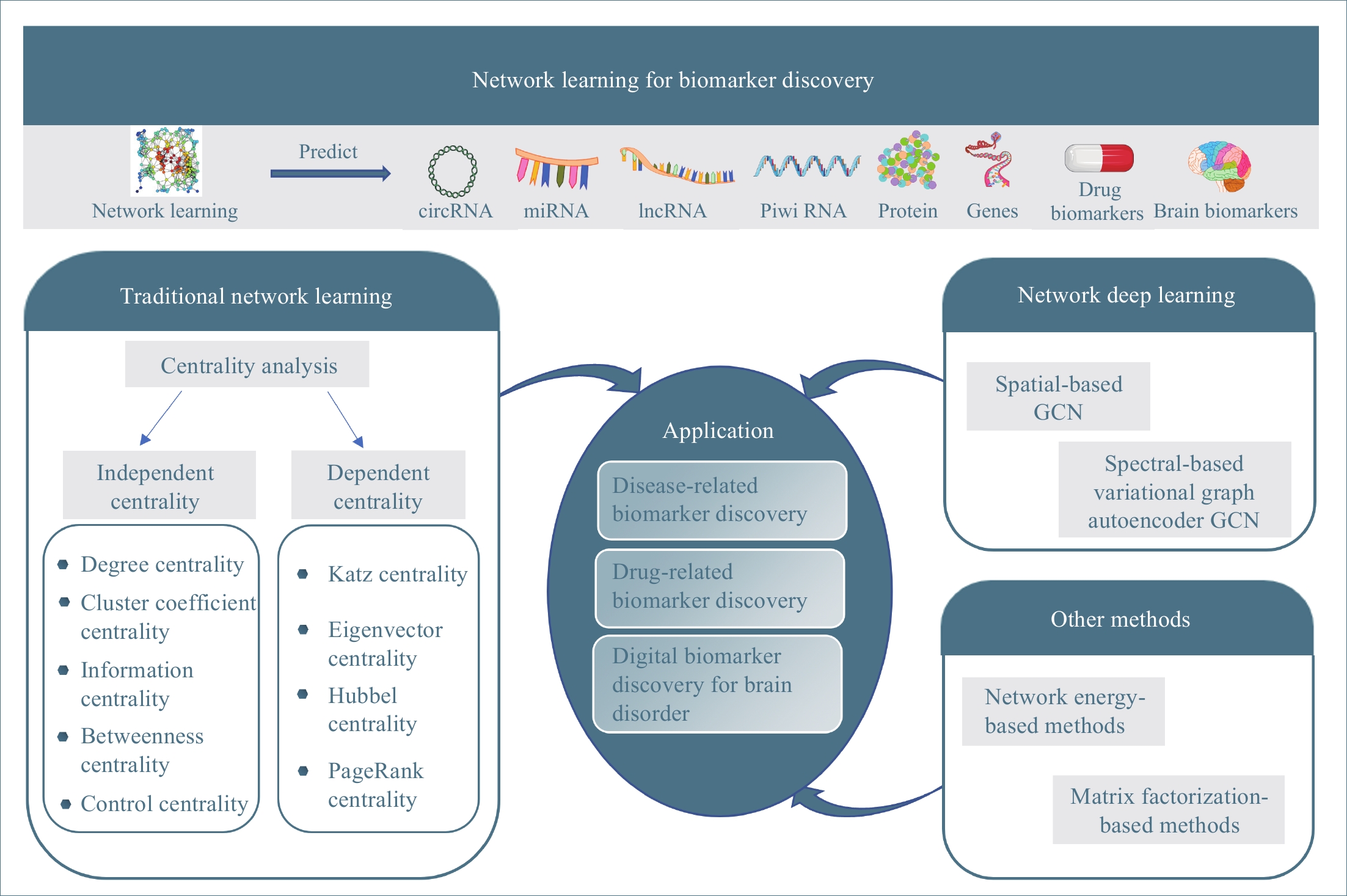
Figure 1. The overview of this study.
2. Traditional Network Learning
In this section, we overview traditional network learning methods with a focus on the centrality-based methods for learning the importance or the specialty of the network elements, as well as their applications in computational medicine for biomarker discovery.
2.1. Centrality Analysis
Centrality indices are to quantify an intuitive feeling that some network elements are more important than others in networks. We classify centrality indices in the literature [22, 23] into two categories: independent centrality and dependent centrality. The independent centrality of a network element is independent of the centrality of other network elements in the network while the dependent centrality of a network element depends on the centrality of all network elements in the network.
2.1.1. Independent Centrality
Although many different centrality indices have been proposed in the literature [22, 23], some of them have certain overlaps for learning knowledge. In the following, we first introduce some widely used independent centrality indices with the least overlap, including degree centrality, cluster coefficient centrality, information centrality, betweenness centrality, and control centrality.
(1) Degree Centrality and Strength
The simplest centrality is the degree centrality  of a vertex
  in an undirected graph
  where
where  is the number of edges in
  that has vertex
  as an endvertex. In a directed network
  , two variants of the degree centrality may be appropriate: the in-degree centrality
  and the out-degree centrality
  , where
  is the number of edges in
  with the destination of vertex
  while
while  is the number of edges in
  that has the origin of vertex
  . In a weighted undirected network
  , the weighted degree centrality of a vertex
  , which is the sum of weights of edges in
  that has the vertex
  as an endvertex, is called the strength in literature.
(2) Cluster Coefficient Centrality
The clustering coefficient of a vertex  in a network quantifies how close its neighbors are to being a clique (complete graph), and can be defined as

where  is the neighborhood of vertex
  , i.e.,
  and
and  is the number of vertices in
  .
.
(3) Closeness Centrality and Information Centrality
The closeness centrality of vertex  is defined as the reciprocal of the total distance between vertex
  and any other vertex
  as follows

When an undirected network is disconnected, the closeness centrality is useless as its value for all vertices will be zero. To mitigate this drawback, the information centrality has been designed.
The information  that can be transmitted between two vertices
  and
and  is defined as the reciprocal of the topological distance
  , i.e.,
  . The information centrality of the vertex
  is defined as the harmonic average information
  over a network as follows:

which is to measure information that can be transmitted between vertex  and any other vertex in a network. It can be seen that when an undirected network is connected, the closeness centrality of its element is exactly the same as its information centrality. However, when an undirected network is disconnected, the information centrality still makes sense while the closeness centrality does not.
(4) Betweenness Centrality
The betweenness centrality of vertex  can be defined as follows:

where  denotes the number of all shortest paths between vertices
  and
and  that contain vertex
  while
while  denotes the number of all shortest paths between vertices
  and
and  , and thus
  is the fraction of shortest paths between vertices
  and
and  that contain vertex
  . Similarly, the betweenness centrality of edge
  can be defined as follows:

where  denotes the number of all shortest paths between vertices
  and
and  that contain edge
  while
while  denotes the number of all shortest paths between vertices
  and
and  , and thus
  is the fraction of shortest paths between vertices
  and
and  that contain edge
  .
.
(5) Control Centrality
Letting  be the
  adjacent matrix of a network, the control centrality of vertex
  can be defined as follows [24,25]:

where  is the
  -th column of the
  identity matrix. The control centrality measures the controllability [26] of a node on which a control signal is actuated.
A vertex is called a hub if its centrality value in a network is relatively higher than a user-specified threshold. For different centralities, different sets of hubs may be produced from the same network. For a network  and any centrality
  , we can define the global centrality of
  as follows:

2.1.2. Dependent Centrality
The independent centralities of one vertex are independent of other vertices. Actually, it is reasonable that the more central a vertex is, the more central its neighbors are and vice versa. This kind of measure is called the dependent centrality. In the following, centrality values are denoted as vectors, each of whose component is corresponding to the centrality of one vertex in the network. All dependent centralities are typically calculated by solving linear systems.
(1) Katz Centrality
The Katz centrality is to measure the impact of a vertex  on any vertex
  of a network. Intuitively, vertex
  can impact on any vertex
  if there is a path from vertex
  to vertex
  . In addition, the longer the path between two vertices
  and
and  is, the smaller the impact of vertex
  on
on  should be. To take the effect of path length into consideration, a damping factor
  is introduced. As a result, the Katz centrality (
  ) can be mathematically defined as follows:

where  is the adjacency matrix of the network. Note that
  is the number of paths from vertex
  to vertex
  with the length of
  . In the matrix-vector format, we have

where  is the
  -dimensional vector where every entry is
  . Let
. Let  be the largest eigenvalue of matrix
  , which is a positive number, and let
  . Then, we have

(2) Eigenvector Centrality
Eigenvector centrality assumes that the centrality value  of vertex
  depends on the values of each adjacent vertex, specifically it is proportional to the sum of the values of each adjacent vertex. Therefore, in the matrix-vector format we have the following equation:

where  . It can be proved that if a network is undirected and connected, then the largest eigenvalue
  of
of  is simple and all entries of the eigenvector corresponding to
  are of the same sign. Therefore, the eigenvector centrality is computed as the scaled eigenvector corresponding to
  .
.
(3) Hubbel Centrality
Further to the eigenvector centrality, Hubbel also took some prior preference information about the centrality value (represented by a column vector  ) into account. As a result, the Hubbel centrality
  satisfies the following equation

If there is no specific prior preference information,  can be taken as
  . Then, we have

which is the same as the Katz centrality for undirected networks.
(4) PageRank Centrality
The initial PageRank centrality  can be viewed as the extension of the eigenvalue centrality by taking the degree of neighbor vertices into account as follows:

where  is the PageRank centrality value of vertex
  and
and  is a proportional constant.
  is the out degree of vertex
  and
and  is the set of vertices pointing to vertex
  . In the matrix-vector format, the initial Pagerank centrality can be expressed as

where the transition matrix  is calculated as follows:

Therefore,  is actually the scaled eigenvector of the transition matrix
  . The final PageRank centrality can be viewed as the type of the Hubbel centrality in that the adjacent matrix is replaced with the transition matrix as follows:

The random walk starting with a vertex on a network is actually to calculate the PageRank centrality of that vertex [27, 28]. Especially, random walk-based algorithms, such as node2vec [28], have been widely used for extracting features of vertices in networks. The above presented dependent centralities follow the idea of positive feedback: the centrality of a vertex is higher if it is connected to other high-valued vertices. In addition, the eigenvector centrality is the fundamental dependent centrality as other dependent centrality can be viewed as its generalization in different ways.
2.2.1. Disease-Related Biomarker Discovery
Jeong et al. [29] conclude that the most highly connected proteins in the cell are the most important for its survival. Han et al. [30] define two types of hubs: party hubs and date hubs, based on the degree centrality in PPI networks, and uncover that these hubs play important biological roles. With various other evidence [31, 32] about the relationships between the centrality and biological roles of network elements, many centralities have been applied to learn biological knowledge from biological networks in past decades. Essential proteins are indispensable proteins for supporting cellular life and thus are important biomarkers [9]. The degree centrality, information centrality, betweenness centrality and other dependent centralities have been used to predict essential proteins from PPI networks with great accuracy [33, 34]. The fundamental dependent centrality and eigenvector centrality have been used to predict essential proteins [34–38]. Tang et al. [39] develop a software package to predict essential proteins based on several commonly used centralities, including degree centrality, betweenness centrality, information centrality, and eigenvector centrality, to name a few. Understanding the role of genetics in diseases is one of the most important goals of the biological sciences. However, determining disease-associated genes requires laborious experiments and thus the centrality indices can be used to predict good candidate disease-associated genes before experimental analysis [40]. The random walk can be used to either directly predict disease-related biomarkers [41, 42] or to learn the features of biomarkers for some machine learning-based prediction methods [43, 44]. Recently, Gentili et al. [5] use the random walk to integrate multi-omics data for disease gene prioritization.
2.2.2. Drug-Related Biomarker Discovery
Traditional drug discovery strategies are not only high monetary-demanding, but also time-consuming. Drug repositioning (also called drug repurposing) is now becoming an effective drug discovery strategy, which involves the investigation on existing drugs for treating different diseases [45]. In drug repositioning [46, 47], a key is to select a list of genes called the gene signature to represent a disease. By placing genes in proper networks, a number of centralities have been used to create gene signatures [48, 49] from gene networks. Drug targets, which are important biomarkers, can be interpreted as steering nodes in controlled biomolecular networks while drugs are viewed as the control signals. Wu et al. [50] develop some seminal theories for the controllability of complex biomolecular networks and design several variants of the control centrality, which have been applied to identify drug targets from regulatory biological networks [51–53].
2.2.3. Digital Biomarkers for Brain Disorders
Interconnections of structurally segregated and functionally specialized regions of the human cerebral cortex can be represented by structural brain networks based on structural brain images [54–57]. The analysis of the large-scale structural brain networks has revealed that brain regions within the structural core share with high degree, strength, and betweenness centrality [58]. Both remitted geriatric depression (RGD) and amnestic mild cognitive impairment (aMCI) are associated with a high risk of developing Alzheimer's Disease (AD). The analysis of structural brain networks with several centralities finds some direct evidence for the association of a great majority of convergent connectivity and a minority of divergent connectivity between RGD and aMCI patients, which may lead to increased attention in defining a population at risk of AD [59]. Gu et al. [60] apply the control centrality to structural brain networks to the region of brains with special cognitive functions, which can be potential target regions for treating brain disorders. With the proper parcellation scheme of the human cerebral cortex, functional brain networks can be constructed based on functional brain magnetic resonance imaging (MRI) images [61]. Mostafa et al. [62] and Yin et al. [63] define the features of patients from their functional brain networks by integrating the centralities with other information to develop the methods for diagnosis of autism spectrum disorder.
3. Network Deep Learning
Convolutional neural network (CNN)-based deep learning has been very successful in the computer vision domain and natural language processing domain as the imaging data and text data are well structured and the neighborhood for the convolutional operation is obvious. By utilizing the neighborhood relations of vertices in a network (graph) [64] for the convolutional operation, the numerous types of graph convolutional networks (GCNs) [65, 66] have been proposed, which can be classified as spatial-based GCNs and spectral-based GCNs.
3.1. Spatial-Based GCN
Analogous to the convolutional operation of a conventional CNN on an image, the spatial-based graph convolutions convolve the features of a central vertex with the features of its neighbors to derive the updated features for the central vertex. The spatial graph convolutional operation essentially propagates vertex information along edges across a whole graph. The graph convolution for vertex  at the
  th layer is designed as [67]:


where  is the feature vector of vertex
  at the
  th layer, and
  is a mediate vector with the same dimension as
  .
.  is the set of all neighbor vertices of vertex
  ,
,  is the number of vertices in
  ,
,  is an activation function and
  is the weight matrix for vertices with the same degree as
  at the
  th layer. However, for large graphs, the number of unique values of vertex degree is often very large. Consequently, there are too many weight matrices to be learned at each layer, possibly leading to the overfitting problem.
In addition, as the number of neighbors of a vertex can vary from one to a thousand or even larger, it is inefficient to take the full size of a vertex’s neighborhood. GraphSage [68] adopts sampling to obtain a fixed number of neighbors for each node and replaces Equation (19) by a general aggregate operation, and the graph convolution is performed by


where  is an aggregation function at the
  th layer, and
  is a random sample of the node
  ’s neighbors. The aggregation function should be invariant to the permutations of node orderings such as a mean, sum or max function [65, 69]. Note that in Equation (22) the weight matrix
  does not depend on the vertex degree. As a result, the number of learnable parameters is greatly reduced and the overfitting problem can be mitigated.
3.2. Spectral-Based Variational Graph Autoencoder
The autoencoder (AE) and its variant variational autoencoder(VAE) are effective tools to learn the hidden features from raw data (or features) [70]. Kipf and Welling [71] propose a two-layer variational graph autoencoder (VGAE) that extends VAE to graphs for the first time. Consider an undirected, unweighted graph  with
with  vertices nodes. Let A be the adjacency matrix of
  and
and  be its degree matrix. Furthermore, let
  be an
be an  matrix consisting of hidden features of all vertices to be learned and
  be an
be an  matrix consisting of raw features of all vertices. VGAE includes two parts: the inference model and generative model, as follows [71].
3.2.1. Inference Model

where  is the matrix of mean vectors
  , similarly
  . The two layer spectral-based GCN is defined as
  with the weight matrices
  .
.  and
and  share the first layer parameters
  .
.  and
and  is the symmetrically normalized adjacency matrix.
3.2.2. Generative Model

where  is the logistic sigmoid function. The VGAE optimizes the variational lower bound
  with respect to the parameters
  :
:

where  is the Kullback-Leibler divergence between two distributions
  and
and  and a Gaussian prior
As GCNs can capture the nonlinear relationship among diseases, drugs and biomarkers in biological networks, more and more GCN-based methods have been proposed for biomarker discovery.
Singh and Lio [72] propose a constrained VGAE variant for predicting disease-gene associations. Wang X. et al. [73] define a new cluster loss function and a dropout mechanism based on the GCN and graph embedding method to improve the generalization ability for predicting gene-disease associations. In order to analyze the underlying mechanism of cancer, Schulte-Sasse et al. [74] design GCNs for classifying and predicting cancer genes. Cai et al. [75] propose a GCN based on fine-grained edge dropout and coarse-grained node dropout to reduce the over-fitting in sparse graphs for predicting synthetic lethality in human cancers. Chereda et al. [76] combine the PPI network and gene expression data for patients and utilize GCN to classify the vertices in the patient’s sub-network for predicting breast cancer metastasis. Rhee et al. [77] propose a hybrid approach of relation networks and localized graph convolutional filtering for breast cancer subtype classification.
3.2.4.
Pan and Shen [78] propose a semi-supervised multi-label graph convolution model (DimiG), which does not rely on known association information between miRNAs and diseases to indirectly predict the association between miRNAs and diseases. Li J. et al. [79] design a GCN to learn the feature representations of miRNAs and diseases from the miRNA functional similarity network and disease semantic similarity network, respectively, to predict all miRNAs related to breast cancer without any known related miRNAs. Li C. et al. [80] integrate miRNA disease, miRNA gene, disease–gene, and PPI networks to extract the features for predicting miRNA disease associations. Using the FastGCN algorithm and the Forest by Penalizing Attributes (Forest PA) classifier, Wang L. et al. [81] can accurately predict potential circRNA disease associations. Wu et al. [82] propose a graph autoencoder to learn the feature representation of lncRNAs and diseases from the bipartite graph associated with lncRNA disease, and the score of the lncRNA disease interaction was calculated from the inner product of the two potential factor vectors. Ding et al. [83] use VGAE to learn the features of miRNAs and diseases from the heterogeneous networks consisting of miRNA similarity network, disease similarity network and known miRNA disease association network for predicting potential miRNA disease associations. In the prediction of disease-related RNAs with limited known data, the integration of multi-view information can help us understand complex biological networks more comprehensively. Ding et al. [84] further design a multi-view VGAE, combined with matrix factorization to predict potential miRNA-disease associations. In addition, the Laplacian matrices are incorporated with a deep factorization machine to predict miRNA-disease associations [85].
When a drug is taken with another drug, the expected efficacy of drugs may be significantly changed. Therefore, research on drug-drug interaction (DDI) is essential to reduce the occurrence of adverse drug events and maximize the synergistic benefits in the treatment of diseases. Zitnik et al. [94] predict the side effects between drugs from a multi-modal heterogeneous network consisting of PPI, drug-protein targets, and drug-drug interactions, where each side effect is represented by a different edge. Ma et al. [95] propose a framework of a multi-view drug graph encoder based on the attention mechanism, which is used to measure the drug similarity. Wang F. et al. [96] propose a GCN with multiple graph kernels for predicting drug-drug interactions.
3.2.5. Image Biomarker Discovery for Brain Disorders
Before GCNs are introduced, CNN-based image analysis has been widely used in various studies, especially in brain image analysis [97–100]. Actually, image data can be represented as a graph structure appropriate for the use of GCNs. Therefore, GCNs have many applications in the field of medical imaging analysis. Parisot et al. [101] propose a framework to exploit GCN and involves representing populations as a sparse graph, where its vertices are associated with imaging-based feature vectors, while phenotypic information is integrated as edge weights and applied to study autism spectrum disorder and Alzheimer’s disease. Gopinath et al. [102] propose an approach to enable direct learning of surface data across compatible surface bases and its superiority is illustrated with applications to brain parcellation.
Ktena et al. [103] exploit concepts of graph convolutions to estimate the similarity between irregular graphs which is alter applied to study the structural or functional connections within the brain. Zhai et al. [104] construct a generative model using graph convolution and VAE to predict the abnormal areas of pulmonary artery-vein. In order to lift the restrictions of fixed graphic structure for a model, Zhang and Pierre [105] propose a spatial GCN-based learning model to classify different brain connections and predict the association between brain connection sub-networks and diseases. Yang et al. [106] integrate different modalities of medical imaging (both brain structural and functional MRIs) with GCNs for predicting bipolar disorder.
The accurate structure prediction can fully clarify the biological mechanism of protein action on a molecular scale, and its application in drug development is of great significance. However. Compared to CNN-based methods, GCN-based methods have shown more powerful capabilities in learning the effective structure of proteins from simplified graphical representations [86]. Zamora-Resendiz and Crivelli [87] propose a spatial GCN for learning protein structures with the natural spatial representation of molecular structures. Gligorijevic et al. [88] model the protein structure as a graph to predict the protein function based on GCNs. Feng et al. [89] introduce a GCN into drug target identification by learning the molecular structure information of drugs. Tran et al. [90] propose a GCN-based framework to learn representations of the drugs and targets for predicting drug-target interactions.
The combination of genomics data and drug information for drug response prediction has promoted the development of personalized medicine. Huang et al. [91] combine a GCN with an autoencoder to predict the association between miRNA and drug resistance. Liu Q. et al. [92] predict the therapeutic effect of drugs on cancer cells by constructing a cancer cell information sub-network and a drug structure sub-network. Considering the complexity of cancer factors, Singha et al. [93] integrate biological network, genomics, inhibitor analysis, and disease–gene association data into large heterogeneous networks. Multiple graph convolution blocks and attention propagation are used for predicting the effect of pharmacotherapy.
4. Other Methods
4.1. Network Energy-Based Methods
Consider a network  with some of its vertices labelled as
  or
or  and others unlabelled vertices. Based on Boltzmann principle and Ising model in the statistic physics, Chen et al. define the network energy with vertex labels and edges and then develop the network energy-based method for calculating the possibility of vertex
  being labeled as
  , as follows [3].

where  and
and  are the numbers of neighbors of vertex
  with label
  and
and  , respectively, and can be calculated as

where  is the labelled value of vertex
  and
and  is the
  -entry of the adjacent matrix of the network.
Network energy-based centrality can be viewed as the extension of classical vitality measures as it quantifies the difference of the network energy between two possible labels of a network element. Different from previously introduced centrality, the network energy-based methods contain the trainable parameters  , and
, and  . In addition, as the network energy is a scalar, the energy of multiple networks can be added together. Therefore, the network energy-based methods on a single network can be straightforwardly extended to multiple networks [3, 4].
Chen et al. have applied the network energy-based methods based on both single network and multiple networks to identify disease-associated genes [3, 107–109]. Note that in Equation (26), only the information of direct neighbors of vertex  is used. To take the information of indirect neighbors into account, Chen et al. design a network energy-based method with a network kernel for identifying disease genes [110]. Let
  be the learnable parameter vector and
  be the feature vector of vertex
  . Then, network energy-based method (26) can be expressed as follows:

Luo et al. define the vertex feature vector different from  and use the generalized centrality with the expression of Equation (28) to predict disease genes [111, 112]. Ding et al. use the random walk to get the features of vertices and use the expression Equation (28) to predict disease-associated circRNAs [43].
4.2. Matrix Factorization-Based Methods
As the entries of the adjacent matrix of an unweighted network are either  or
or  , the adjacent matrices can be viewed as nonnegative matrices. Therefore, the nonnegative matrix factorization (NMF) can be used to learn the features of network elements as inputs of machine learning methods for downstream analysis. Mathematically, given a nonnegative matrix
  , and a positive integer
  , NMF tries to find two nonnegative matrices
  and
and  such that

There are several ways to measure the best approximation of  by
by  , one of which has widely been used is minimizing the Euclidean distance between
  and
and  as follows [113, 114]:

where  is the Frobenius norm of a matrix and
  stands for "entry-wise greater or equal to zero". Each row vector of matrices
  and
and  can be explained as the feature vector network vertices. For example, consider
  to be the adjacent matrix of the associate network of
  diseases and
  genes. Then, the
  -th row vector of matrix
  is the
  -dimensional feature vector of disease
  while the
  -th row vector of matrix
  is the
  -dimensional feature vector of gene
  . In the literature, NMF is often used for learning the features of network elements for clustering [115–117].
 could be a symmetric matrix when it presents the adjacent matrix of interaction networks such as PPI networks [16] and (DDI) networks [17]. Then, symmetrical nonnegative matrix factorization method [118] can be used to learn the features of network elements. The optimization formulation of NMF (27) can also integrate other information about the elements of a network to learn more reasonable features. For example, let
  be the adjacent matrix of the similarity network for elements corresponding to rows in
  while
while  be the adjacent matrix of the similarity network for elements corresponding to columns in
  . Then, the optimization problem can be formulated as follows:

where  is the trace of a matrix.
  and
and  are the Laplace matrice of the similarity networks for elements corresponding to rows and columns, respectively.
In the early years, Pascual-Montano et al. develop a software package for NMF and applications in biology [119] while Tian et al. review the matrix decomposition methods in bioinformatics [120], which includes NMF and applications for biomarker discovery. Recently, Fujita et al. integrate NMF and pathway signature analysis for biomarker discovery [121]. Jamali et al. develop NMF methods for predicting drug-related biomarkers (microRNA) [122] and proteins [123]. Luo et al. apply NMF to predict disease-related biomarkers (genes) [124]. Lin and Ma predict disease-related biomarkers (lncRNA) in heterogeneous networks with co-regularized NMF [125]. Peng et al. develop Rnmflp for predicting disease-related biomarkers (circRNAs) based on robust NMF and label propagation [126].
NMF of adjacent matrices of networks has been extended in two different ways for biomarker discovery. Traditional NMF only involves the multiplications and additions, which is called linear factorization, and only has one hidden layer [70]. One way to extend the linear NMF is to introduce nonlinear factorization. Bayesian or logistic matrix factorization [70] is one of the widely used nonlinear NMF for biomarker discovery. Chen et al. use Bayesian NMF for predicting disease-related biomarkers (miRNA) [127]. Furthermore, Ding et al. develop a deep belief network-based matrix factorization model with multiple layers and nonlinear transformation for predicting disease-related biomarkers (miRNA) [128]. Networks with one or two types of vertices can be represented by planar graphs and their adjacent matrices are two-dimensional tensors. Networks with more than two types of vertices are represented by multi-dimensional graphs and as a result, their adjacent matrices are high-dimensional tensors. Another way to extend NMF for adjacent matrices of networks is to design the nonnegative high-dimensional tensor factorization. Jamali et al. construct a three-dimensional graph with three types of vertices: drugs, targets, and diseases, and develop a nonnegative tensor decomposition method for drug repositioning [129].
5. Discussions and Future Directions
A pair of vertices in a network, which forms an edge, could play a very important role in many biological processes, including the development of diseases [130]. The studies in [9] show that synthetic lethality between two genes can personalize targeted therapies. Most centralities for vertices can be also defined for edges, and edge centralities have been used to predict essential proteins [131]. Luo et al. [132] use the random walk (node2vec) to learn the features of disease gene association from networks for a deep learning model to predict disease-related biomarkers. However, compared to vertex centralities, edge centralities have been paid much less attention to in the existing literature of network learning. Therefore, network learning for edges can be a promising direction for drug discovery. If genes are mapped in some proper networks, the lethality between two genes can be viewed to study the centralities of edges in such networks.
Biological networks are typically dynamics. For example, some edges appearing at one-time point (or subcellular localization) may disappear at another time point (or one subcellular localization) in PPI networks [133–135]. The traditional centrality-based methods have been applied to dynamic biological networks to learn the knowledge for biomarker discovery [136, 137]. Another promising direction for network learning is to combine dynamic biological networks with deep neural networks to learn the properties or features of network elements for drug discovery. Network biology is useful for modeling complex biological phenomena [138] and has attracted attention with the advent of novel network (especially deep) learning methods. Similar to other deep learning methods, network deep learning often suffers from the lack of interpretability. However, the interpretability of network learning models could be the top priority in the domain of biomarker discovery. The third promising direction is to increase the interpretability of network deep learning models for biomarker discovery by incorporating more biological knowledge into models.
Author Contributions: Fang-Xiang Wu: conceptualization, investigation, writing—original draft preparation, writing—review and editing, supervision, project administration and funding acquisition; Yulian Ding: investigation, writing—original draft preparation, writing—review and editing, visualization; Minghan Fu: investigation, writing—review and editing; Ping Luo: investigation and writing—review and editing. All authors have read and agreed to the published version of the manuscript.
Funding: This work is supported in part by Natural Science and Engineering Research Council of Canada (NSERC).
Conflicts of Interest: The authors declare no conflict of interest.
References
- Fournier, J.C. Graphs Theory and Applications: With Exercises and Problems; Wiley-ISTE: London, 2009.
- Li, A.S.; Li, J.K.; Pan, Y.C.; et al. Homophyly/kinship model: Naturally evolving networks. Sci. Rep., 2015, 5: 15140.
- Chen, B.L.; Wang, J.X.; Li, M.; et al. Identifying disease genes by integrating multiple data sources. BMC Med. Genomics, 2014, 7: S2.
- Li, Y.F.; Wu, F.X.; Ngom, A. A review on machine learning principles for multi-view biological data integration. Briefings Bioinf., 2018, 19: 325−340.
- Gentili, M.; Martini, L.; Sponziello, M.; et al. Biological random walks: Multi-omics integration for disease gene prioritization. Bioinformatics, 2022, 38: 4145−4152.
- Lewis, T.G. Network Science: Theory and Applications; John Wiley & Sons, Inc.: New Jersey, 2009.
- Težak, Ž.; Kondratovich, M.V.; Mansfield, E. Us FDA and personalized medicine: In vitro diagnostic regulatory perspective. Pers. Med., 2019, 7: 517−530.
- OMIM. An Online Catalog of Human Genes and Genetic Disorders. Available online: https://omim.org/ (accessed on 12 October 2022).
- Parameswaran, S.; Kundapur, D.; Vizeacoumar, F.S.; et al. A road map to personalizing targeted cancer therapies using synthetic lethality. Trends Cancer, 2019, 5: 11−29.
- Goh, K.I.; Cusick, M.E.; Valle, D.; et al. The human disease network. Proc. Natl. Acad. Sci. USA, 2007, 104: 8685−8690.
- Vidal, M.; Cusick, M.E.; Barabási, A.L. Interactome networks and human disease. Cell, 2011, 144: 986−998.
- Oti, M.; Brunner, H.G. The modular nature of genetic diseases. Clin Genet, 2007, 71: 1−11.
- Yıldırım, M.A.; Goh, K.I.; Cusick, M.E.; et al. Drug-target network. Nat Biotechnol, 2007, 25: 1119−1126.
- Bullmore, E.; Sporns, O. Complex brain networks: Graph theoretical analysis of structural and functional systems. Nat. Rev. Neurosci., 2009, 10: 186−198.
- Jones, S.; Thornton, J.M. Principles of protein-protein interactions. Proc. Natl. Acad. Sci. USA, 1996, 93: 13−20.
- Venkatesan, K.; Rual, J.F.; Vazquez, A.; et al. An empirical framework for binary interactome mapping. Nat. Methods, 2009, 6: 83−90.
- Wishart, D.S.; Feunang, Y.D.; Guo, A.C.; et al. Drugbank 5.0: A major update to the drugbank database for 2018. Nucleic Acids Res., 2018, 46: D1074−D1082.
- Ideker, T.; Krogan, N.J. Differential network biology. Mol. Syst. Biol., 2012, 8: 565.
- Oughtred, R.; Stark, C.; Breitkreutz, B.J.; et al. The biogrid interaction database: 2019 update. Nucleic Acids Res., 2019, 47: D529−D541.
- Gysi, D.M.; do Valle, Í.; Zitnik, M.; et al. Network medicine framework for identifying drug-repurposing opportunities for COVID-19. Proc. Natl. Acad. Sci. USA, 2021, 118: e2025581118.
- Guney, E.; Menche, J.; Vidal, M.; et al. Network-based in silico drug efficacy screening. Nat. Commun., 2016, 7: 10331.
- Brandes, U.; Erlebach, T. Network Analysis: Methodological Foundations; Springer: Berlin, Heidelberg, 2005. doi: 10.1007/b106453
- Latora, V.; Nicosia, V.; Russo, G. Complex Networks: Principles, Methods and Applications; Cambridge University Press: Cambridge, 2017.
- Liu, Y.Y.; Slotine, J.J.; Barabási, A.L. Control centrality and hierarchical structure in complex networks. PLoS One, 2012, 7: e44459.
- Wu, L.; Li, M.; Wang, J.X.; et al. Cytoctrlanalyser: A cytoscape app for biomolecular network controllability analysis. Bioinformatics, 2018, 38: 1428−1430.
- Liu, Y.Y.; Slotine, J.J.; Barabási, A.L. Controllability of complex networks. Nature, 2011, 473: 167−173.
- Göbel, F.; Jagers, A.A. Random walks on graphs. Stoch. Process. Their Appl., 1974, 2: 311−336.
- Grover, A.; Leskovec, J. node2vec: Scalable feature learning for networks. In Proceedings of the 22nd ACM SIGKDD International Conference on Knowledge Discovery and Data Mining, San Francisco, 13 August 2016; ACM: San Francisco, 2016; pp. 855–864. doi: 10.1145/2939672.2939754
- Jeong, H.; Mason, S.P.; Barabási, A.L.; et al. Lethality and centrality in protein networks. Nature, 2001, 411: 41−42.
- Han, J.D.J.; Bertin, N.; Hao, T.; et al. Evidence for dynamically organized modularity in the yeast protein–protein interaction network. Nature, 2004, 430: 88−93.
- Wu, X.B.; Jiang, R.; Zhang, M.Q.; et al. Network-based global inference of human disease genes. Mol. Syst. Biol., 2008, 4: 189.
- Ramirez, F.; Schlicker, A.; Assenov, Y.; et al. Computational analysis of human protein interaction networks. Proteomics, 2007, 7: 2541−2552.
- Peng, W.; Wang, J.X.; Wang, W.P.; et al. Iteration method for predicting essential proteins based on orthology and protein-protein interaction networks. BMC Syst. Biol., 2012, 6: 87.
- Li, M.; Zhang, H.H.; Wang, J.X.; et al. A new essential protein discovery method based on the integration of protein-protein interaction and gene expression data. BMC Syst. Biol., 2012, 6: 15.
- Mistry, D.; Wise, R.P.; Dickerson, J.A. DiffSLC: A graph centrality method to detect essential proteins of a protein-protein interaction network. PLoS One, 2017, 12: e0187091.
- Elahi, A.; Babamir, S.M. Identification of essential proteins based on a new combination of topological and biological features in weighted protein–protein interaction networks. IET Syst. Biol., 2018, 12: 247−257.
- Junker, B.H.; Koschützki, D.; Schreiber, F. Exploration of biological network centralities with centiBiN. BMC Bioinformatics, 2006, 7: 219.
- Grassler, J.; Koschützki, D.; Schreiber, F. CentiLiB: Comprehensive analysis and exploration of network centralities. Bioinformatics, 2012, 28: 1178−1179.
- Tang, Y.; Li, M.; Wang, J.X.; et al. CytoNCA: A cytoscape plugin for centrality analysis and evaluation of protein interaction networks. Biosystems, 2015, 127: 67−72.
- Özgür, A.; Vu, T.; Erkan, G.; et al. Identifying gene-disease associations using centrality on a literature mined gene-interaction network. Bioinformatics, 2008, 24: i277−i285.
- Wei, P.J.; Wu, F.X.; Xia, J.F.; et al. Prioritizing cancer genes based on an improved random walk method. Front. Genet., 2020, 11: 377.
- Li, Y.J.; Li, J.Y. Disease gene identification by random walk on multigraphs merging heterogeneous genomic and phenotype data. BMC Genomics, 2012, 13: S27.
- Ding, Y.L.; Chen, B.L.; Lei, X.J.; et al. Predicting novel CircRNA-disease associations based on random walk and logistic regression model. Comput. Biol. Chem., 2020, 87: 107287.
- Chen, X.; Liu, M.X.; Yang, G.Y. RWRMDA: Predicting novel human microRNA-disease associations. Mol. BioSyst., 2012, 8: 2792−2798.
- Ashburn, T.T.; Thor, K.B. Drug repositioning: Identifying and developing new uses for existing drugs. Nat. Rev. Drug Discov., 2004, 3: 673−683.
- Lamb, J.; Crawford, E.D.; Peck, D.; et al. The connectivity map: Using gene-expression signatures to connect small molecules, genes, and disease. Science, 2006, 313: 1929−1935.
- Fei, W.; Lei, X.J.; Wu, F.X. A review of drug repositioning based chemical-induced cell line expression data. Curr. Med. Chem., 2020, 27: 5340−5350.
- Wang, F.; Ding, Y.L.; Lei, X.J.; et al. Identifying gene signatures for cancer drug repositioning based on sample clustering. IEEE/ACM Trans. Comput. Biol. Bioinf., 2022, 19: 953−965.
- Huang, C.H.; Chang, P.M.H.; Hsu, C.W.; et al. Drug repositioning for non-small cell lung cancer by using machine learning algorithms and topological graph theory. BMC Bioinformatics, 2016, 17: S2.
- Wu, F.X.; Wu, L.; Wang, J.X.; et al. Transittability of complex networks and its applications to regulatory biomolecular networks. Sci. Rep., 2014, 4: 4819.
- Wu, L.; Li, M.; Wang, J.X.; et al. Controllability and its applications to biological networks. J. Comput. Sci. Technol., 2019, 34: 16−34.
- Wu, L.; Tang, L.K.; Li, M.; et al. Biomolecular network controllability with drug binding information. IEEE Trans. NanoBiosci., 2017, 16: 326−332.
- Wu, L.; Shen, Y.C.; Li, M.; et al. Network output controllability-based method for drug target identification. IEEE Trans. NanoBiosci, 2015, 14: 184−191.
- Rudie, J.D.; Brown, J.A.; Beck-Pancer, D.; et al. Altered functional and structural brain network organization in autism. NeuroImage Clin., 2013, 2: 79−94.
- Wang, D.H.; Buckner, R.L.; Fox, M.D.; et al. Parcellating cortical functional networks in individuals. Nat. Neurosci., 2015, 18: 1853−1860.
- Power, J.D.; Cohen, A.L.; Nelson, S.M.; et al. Functional network organization of the human brain. Neuron, 2011, 72: 665−678.
- Liu, J.; Li, M.; Pan, Y.; et al. Complex brain network analysis and its applications to brain disorders: A survey. Complexity, 2017, 2017: 8362741.
- Hagmann, P.; Cammoun, L.; Gigandet, X.; et al. Mapping the structural core of human cerebral cortex. PLoS Biol., 2008, 6: e159.
- Bai, F.; Shu, N.; Yuan, Y.G.; et al. Topologically convergent and divergent structural connectivity patterns between patients with remitted geriatric depression and amnestic mild cognitive impairment. J. Neurosci., 2012, 32: 4307−4318.
- Gu, S.; Pasqualetti, F.; Cieslak, M.; et al. Controllability of structural brain networks. Nat. Commun., 2015, 6: 8414.
- Power, J.D.; Cohen, A.L.; Nelson, S.M.; et al. Functional network organization of the human brain. Neuron, 2011, 72: 665−678.
- Mostafa, S.; Tang, L.K.; Wu, F.X. Diagnosis of autism spectrum disorder based on eigenvalues of brain networks. IEEE Access, 2019, 7: 128474−128486.
- Yin, W.T.; Mostafa, S.; Wu, F.X. Diagnosis of autism spectrum disorder based on functional brain networks with deep learning. J. Comput. Biol., 2021, 28: 146−615.
- Luo, P.; Ding, Y.L.; Lei, X.J.; et al. deepDriver: Predicting cancer driver genes based on somatic mutations using deep convolutional neural networks. Front. Genet., 2019, 10: 13.
- Zhang, S.; Tong, H.H.; Xu, J.J.; et al. Graph convolutional networks: A comprehensive review. Comput. Soc. Netw., 2019, 6: 11.
- Wu, Z.H.; Pan, S.R.; Chen, F.W.; et al. A comprehensive survey on graph neural networks. IEEE Trans. Neural Netw. Learn. Syst., 2021, 32: 4−24.
- Duvenaud, D.; Maclaurin, D.; Aguilera-Iparraguirre, J.; et al. Convolutional networks on graphs for learning molecular fingerprints. In Proceedings of the 28th International Conference on Neural Information Processing Systems, Montreal, 07 December 2015; MIT Press: Montreal, 2015; pp. 2224–2232. doi: 10.5555/2969442.2969488
- Hamilton, W.L.; Ying, R.; Leskovec, J. Inductive representation learning on large graphs. In Proceedings of the 31st International Conference on Neural Information Processing Systems, Long Beach, 04 December 2017; Curran Associates Inc.: Long Beach, 2017; pp. 1025–1035. doi: 10.5555/3294771.3294869
- Zhang, Y.C.; Lei, X.J.; Pan, Y.; et al. Drug repositioning with graphSAGE and clustering constraints based on drug and disease networks. Front. Pharmacol., 2022, 13: 872785.
- Aggarwal, C.C. Neural Networks and Deep Learning: A Textbook; Springer: Cham, Switzerland, 2018. doi: 10.1007/978-3-319-94463-0
- Kipf, T.N.; Welling, M. Variational graph auto-encoders. arXiv: 1611.07308, 2016. Available online: https://arxiv.org/abs/1611.07308(accessed on 11 October 2022).
- Singh, V.; Lio’, P. Towards probabilistic generative models harnessing graph neural networks for disease-gene prediction. arXiv: 1907.05628, 2019. Available online: https://arxiv.org/abs/1907.05628v1(accessed on 12 October 2022).
- Wang, X.C.; Gong, Y.C.; Yi, J.; et al. Predicting gene-disease associations from the heterogeneous network using graph embedding. In Proceedings of 2019 IEEE International Conference on Bioinformatics and Biomedicine, San Diego, 18–21 November 2019; IEEE: San Diego, 2019; pp. 504–511. doi: 10.1109/BIBM47256.2019.8983134
- Schulte-Sasse, R.; Budach, S.; Hnisz, D.; et al. Graph convolutional networks improve the prediction of cancer driver genes. In Proceedings of the 28th International Conference on Artificial Neural Networks, Munich, 17–19 September 2019; Springer: Munich, 2019; pp. 658–668. doi: 10.1007/978-3-030-30493-5_60
- Cai, R.C.; Chen, X.X.; Fang, Y.; et al. Dual-dropout graph convolutional network for predicting synthetic lethality in human cancers. Bioinformatics, 2020, 36: 4458−4465.
- Chereda, H.; Bleckmann, A.; Menck, K.; et al. Explaining decisions of graph convolutional neural networks: Patient-specific molecular subnetworks responsible for metastasis prediction in breast cancer. Genome Med., 2021, 13: 42.
- Rhee, S.; Seo, S.; Kim, S. Hybrid approach of relation network and localized graph convolutional filtering for breast cancer subtype classification. In Proceedings of the Twenty-Seventh International Joint Conference on Artificial Intelligence, Stockholm, 13–19 July 2018; IJCAI.org: Stockholm, 2018; pp. 3527–3534.
- Pan, X.Y.; Shen, H.B. Inferring disease-associated microRNAs using semi-supervised multi-label graph convolutional networks. iScience, 2019, 20: 265−277.
- Li, J.; Zhang, S.; Liu, T.; et al. Neural inductive matrix completion with graph convolutional networks for miRNA-disease association prediction. Bioinformatics, 2020, 36: 2538−2546.
- Li, C.Y.; Liu, H.J.; Hu, Q.; et al. A novel computational model for predicting microRNA-disease associations based on heterogeneous graph convolutional networks. Cells, 2019, 8: 977.
- Wang, L.; You, Z.H.; Li, Y.M.; et al. GCNCDA: A new method for predicting circRNA-disease associations based on graph convolutional network algorithm. PLoS Comput. Biol., 2020, 16: e1007568.
- Wu, X.M.; Lan, W.; Dong, Y.F.; et al. Inferring lncRNA-disease associations based on graph autoencoder matrix completion. Comput. Biol. Chem., 2020, 87: 107282.
- Ding, Y.L.; Tian, L.P.; Lei, X.J.; et al. Variational graph auto-encoders for miRNA-disease association prediction. Methods, 2021, 192: 25−34.
- Ding, Y.L.; Lei, X.J.; Liao, B.; et al. Predicting miRNA-disease associations based on multi-view variational graph auto-encoder with matrix factorization. IEEE J. Biomed. Health Inf., 2022, 26: 446−457.
- Ding, Y.L.; Lei, X.J.; Liao, B.; et al. MLRDFM: A multi-view laplacian regularized deepFM model for predicting miRNA-disease associations. Brief. Bioinform., 2022, 23: bbac079.
- Sun, M.Y.; Zhao, S.D.; Gilvary, C.; et al. Graph convolutional networks for computational drug development and discovery. Brief. Bioinform., 2020, 22: 919−935.
- Zamora-Resendiz, R.; Crivelli, S. Structural learning of proteins using graph convolutional neural networks. bioRxiv 2019, in press. doi: 10.1101/610444
- Gligorijević, V.; Renfrew, P.D.; Kosciolek, T.; et al. Structure-based protein function prediction using graph convolutional networks. Nat. Commun., 2021, 12: 3168.
- Feng, Q.Y.; Dueva, E.; Cherkasov, A.; et al. PADME: A deep learning-based framework for drug-target interaction prediction. arXiv: 1807.09741, 2018. Available online: https://arxiv.org/abs/1807.09741(accessed on 12 October 2022).
- Tran, H.N.T.; Thomas, J.J.; Ahamed Hassain Malim, N.H. DeepNC: A framework for drug-target interaction prediction with graph neural networks. PeerJ, 2022, 10: e13163.
- Huang, Y.A.; Hu, P.W.; Chan, K.C.C.; et al. Graph convolution for predicting associations between miRNA and drug resistance. Bioinformatics, 2020, 36: 851−858.
- Liu, Q.; Hu, Z.Q.; Jiang, R.; et al. DeepCDR: A hybrid graph convolutional network for predicting cancer drug response. Bioinformatics, 2020, 36: i911−i918.
- Singha, M.; Pu, L.M.; Shawky, A.E.M.; et al. GraphGR: A graph neural network to predict the effect of pharmacotherapy on the cancer cell growth. bioRxiv 2020, in press. doi: 10.1101/2020.05.20.107458
- Zitnik, M.; Agrawal, M.; Leskovec, J. Modeling polypharmacy side effects with graph convolutional networks. Bioinformatics, 2018, 34: i457−i466.
- Ma, T.F.; Xiao, C.; Zhou, J.Y.; et al. Drug similarity integration through attentive multi-view graph auto-encoders. In Proceedings of the 27th International Joint Conference on Artificial Intelligence, Stockholm, 13 July 2018; AAAI: Stockholm, 2018; pp. 3477–3483. doi: 10.5555/3304222.3304251
- Wang, F.; Lei, X.J.; Liao, B.; et al. Predicting drug-drug interactions by graph convolutional network with multi-kernel. Brief. Bioinform., 2022, 23: bbab511.
- Liu, L.L.; Heng, J.H.; Quan, Q.; et al. A survey on U-shaped networks in medical image segmentations. Neurocomputing, 2020, 409: 244−258.
- Liu, L.L.; Chen, S.W.; Zhang, F.H.; et al. Deep convolutional neural network for automatically segmenting acute ischemic stroke lesion in multi-modality MRI. Neural Comput. Appl., 2020, 32: 6545−6558.
- Liu, L.L.; Kurgan, L.; Wu, F.X.; et al. Attention convolutional neural network for accurate segmentation and quantification of lesions in ischemic stroke disease. Med. Image Anal., 2020, 65: 101791.
- Liu, L.L.; Wu, F.X.; Wang, Y.P.; et al. Multi-receptive-field CNN for semantic segmentation of medical images. IEEE J. Biomed. Health Inf., 2020, 24: 3215−3225.
- Parisot, S.; Ktena, S.I.; Ferrante, E.; et al. Disease prediction using graph convolutional networks: Application to autism spectrum disorder and Alzheimer’s disease. Med. Image Anal., 2018, 48: 117−130.
- Gopinath, K.; Desrosiers, C.; Lombaert, H. Graph convolutions on spectral embeddings for cortical surface parcellation. Med. Image Anal., 2019, 54: 297−305.
- Ktena, S.I.; Parisot, S.; Ferrante, E.; et al. Distance metric learning using graph convolutional networks: Application to functional brain networks. In Proceedings of the 20th International Conference on Medical Image Computing and Computer-Assisted Intervention, Quebec City, 11–13 September 2017; Springer: Quebec City, 2017; 469–477. doi: 10.1007/978-3-319-66182-7_54
- Zhai, Z.W.; Staring, M.; Zhou, X.H.; et al. Linking convolutional neural networks with graph convolutional networks: Application in pulmonary artery-vein separation. In Proceedings of the First International Workshop on Graph Learning in Medical Imaging, Shenzhen, 14 November 2019; Springer: Shenzhen, 2019; pp. 36–43. doi: 10.1007/978-3-030-35817-4_5
- Zhang, Y.; Bellec, P. Transferability of brain decoding using graph convolutional networks. bioRxiv 2020, in press. doi: 10.1101/2020.06.21.163964
- Yang, H.Z.; Li, X.X.; Wu, Y.F.; et al. Interpretable multimodality embedding of cerebral cortex using attention graph network for identifying bipolar disorder. In Proceedings of the 22nd International Conference on Medical Image Computing and Computer-Assisted Intervention, Shenzhen, 10 October 2019; Springer: Shenzhen, 2019; pp. 799–807. doi: 10.1007/978-3-030-32248-9_89
- Chen, B.L.; Shang, X.Q.; Li, M.; et al. Identifying individual-cancer-related genes by rebalancing the training samples. IEEE Trans. Nanobiosci., 2016, 15: 309−315.
- Chen, B.L.; Shang, X.Q.; Li, M.; et al. A two-step logistic regression algorithm for identifying individual-cancer-related genes. In Proceedings of 2015 IEEE International Conference on Bioinformatics and Biomedicine, Washington, 09–12 November 2015; IEEE: Washington, 2015; pp. 195–200. doi: 10.1109/BIBM.2015.7359680
- Chen, B.L.; Li, M.; Wang, J.X.; et al. A fast and high performance multiple data integration algorithm for identifying human disease genes. BMC Med. Genomics, 2015, 8: S2.
- Chen, B.L.; Li, M.; Wang, J.X.; et al. Disease gene identification by using graph kernels and Markov random fields. Sci. China Life Sci., 2014, 57: 1054−1063.
- Luo, P.; Tian, L.P.; Ruan, J.S.; et al. Disease gene prediction by integrating PPI networks, clinical RNA-SEQ data and OMIM data. IEEE/ACM Trans. Comput. Biol. Bioinform., 2019, 16: 222−232.
- Luo, P.; Tian, L.P.; Ruan, J.S.; et al. Identifying disease genes from PPI networks weighted by gene expression under different conditions. In Proceedings of 2016 IEEE International Conference on Bioinformatics and Biomedicine, Shenzhen, 15-18 December 2016; IEEE: Shenzhen, 2016; pp. 1259–1264. doi: 10.1109/BIBM.2016.7822699
- Wang, Y.X.; Zhang, Y.J. Nonnegative matrix factorization: A comprehensive review. IEEE Trans. Knowl. Data Eng., 2013, 25: 1336−1353.
- Li, L.X.; Wu, L.; Zhang, H.S.; et al. A fast algorithm for nonnegative matrix factorization and its convergence. IEEE Trans. Neural Netw. Learn. Syst., 2014, 25: 1855−1863.
- Shi, Y. Multiclass spectral clustering. In Proceedings of the Ninth IEEE International Conference on Computer Vision, Nice, 13-16 October 2003; IEEE: Nice, 2003; pp. 313–319. doi: 10.1109/ICCV.2003.1238361
- Kumar, A.; Rai, P.; Daumé III, H. Co-regularized multi-view spectral clustering. In Proceedings of the 24th International Conference on Neural Information Processing Systems, Granada, 12 December 2011; Curran Associates Inc.: Granada, 2011; pp. 1413–1421. doi: 10.5555/2986459.2986617
- Bolla, M. Spectral Clustering and Biclustering; Wiley: Chichester, 2013.
- Tiain, L.P.; Luo, P.; Wang, H.Y.; et al. CASNMF: A converged algorithm for symmetrical nonnegative matrix factorization. Neurocomputing, 2018, 275: 2031−2040.
- Pascual-Montano, A.; Carmona-Saez, P.; Chagoyen, M.; et al. bioNMF: A versatile tool for non-negative matrix factorization in biology. BMC Bioinformatics, 2006, 7: 366.
- Tian, L.P.; Liu, L.Z.; Wu, F.X. Matrix decomposition methods in bioinformatics. Curr. Bioinform, 2013, 8: 259−266.
- Fujita, N.; Mizuarai, S.; Murakami, K.; et al. Biomarker discovery by integrated joint non-negative matrix factorization and pathway signature analyses. Sci. Rep., 2018, 8: 9743.
- Jamali, A.A.; Kusalik, A.; Wu, F.X. MDIPA: A microRNA-drug interaction prediction approach based on non-negative matrix factorization. Bioinformatics, 2020, 36: 5061−5067.
- Jamali, A.A.; Kusalik, A.J.; Wu, F.X. NMTF-DTI: A nonnegative matrix tri-factorization approach with multiple kernel fusion for drug-target interaction prediction. IEEE/ACM Trans. Comput. Biol. Bioinform., 2021, in press. doi: 10.1109/TCBB.2021.3135978
- Luo, P.; Xiao, Q.H.; Wei, P.J.; et al. Identifying disease-gene associations with graph-regularized manifold learning. Front. Genet., 2019, 10: 270.
- Lin, Y.; Ma, X.K. Predicting lincRNA-disease association in heterogeneous networks using co-regularized non-negative matrix factorization. Front. Genet., 2021, 11: 622234.
- Peng, L.; Yang, C.; Huang, L.; et al. RNMFLP: Predicting circRNA-disease associations based on robust nonnegative matrix factorization and label propagation. Brief. Bioinform., 2022, 23: bbac155.
- Chen, X.; Li, S.X.; Yin, J.; et al. Potential miRNA-disease association prediction based on kernelized Bayesian matrix factorization. Genomics, 2020, 112: 809−819.
- Ding, Y.L.; Wang, F.; Lei, X.J.; et al. Deep belief network-based matrix factorization model for microRNA-disease associations prediction. Evol. Bioinform., 2020, 16: 1176934320919707.
- Jamali, A.A.; Tan, Y.T.; Kusalik, A.; et al. NTD-DR: Nonnegative tensor decomposition for drug repositioning. PLoS One, 2022, 17: e0270852.
- Wang, X.J.; Gulbahce, N.; Yu, H.Y. Network-based methods for human disease gene prediction. Brief. Funct. Genomics, 2011, 10: 280−293.
- Wang, J.X.; Li, M.; Wang, H.; et al. Identification of essential proteins based on edge clustering coefficient. IEEE/ACM Trans. Comput. Biol. Bioinform., 2012, 9: 1070−1080.
- Luo, P.; Li, Y.Y.; Tian, L.P.; et al. Enhancing the prediction of disease-gene associations with multimodal deep learning. Bioinformatics, 2019, 35: 3735−3742.
- Chen, B.L.; Fan, W.W.; Liu, J.; et al. Identifying protein complexes and functional modules—from static PPI networks to dynamic PPI networks. Brief. Bioinform., 2014, 15: 177−194.
- Wang, J.X.; Peng, X.Q.; Peng, W.; et al. Dynamic protein interaction network construction and applications. Proteomics, 2014, 14: 338−352.
- Meng, X.M.; Li, M.; Wang, J.X.; et al. Construction of the spatial and temporal active protein interaction network for identifying protein complexes. In Proceedings of 2016 IEEE International Conference on Bioinformatics and Biomedicine, Shenzhen, 15–18 December 2016; IEEE: Shenzhen, 2016; pp. 631–636. doi: 10.1109/BIBM.2016.7822592
- Xiao, Q.H.; Wang, J.X.; Peng, X.Q.; et al. Identifying essential proteins from active PPI networks constructed with dynamic gene expression. BMC Genomics, 2015, 16 Suppl 3: S1.
- Zhang, W.; Xu, J.; Li, Y.Y.; et al. Detecting essential proteins based on network topology, gene expression data, and gene ontology information. IEEE/ACM Trans. Comput. Biol. Bioinform., 2018, 15: 109−116.
- Guo, M.G.; Sosa, D.N.; Altman, R.B. Challenges and opportunities in network-based solutions for biological questions. Brief. Bioinform., 2022, 23: bbab437.