

Downloads
Download


This work is licensed under a Creative Commons Attribution 4.0 International License.
Article
Time-Dependent Vehicle Speed Variation Based Global Path Planning for Intelligent Connected Vehicles
Sihao Chen 1,2, Zhenfeng Wang 1,2, Zhengbai Liu 3, Xianyi Yang 1,2, and Heng Wang 1,2,*
1 College of Mechanical and Electrical Engineering, Henan Agricultural University, Zhengzhou 450002, China
2 Henan Provincial Cold Chain Information and Equipment Laboratory for Logistics of Agricultural Products, Zhengzhou 450002, China
3 College of Innovation and Entrepreneurship, Southern University of Science and Technology, Shenzhen 518055, China
* Correspondence: dawn.wangh@henau.edu.cn
Received: 8 May 2023
Accepted: 30 May 2023
Published: 21 June 2023
Abstract: When an intelligent connected vehicle (ICV) autonomously completes an intelligent driving assignment, the decision planning layer needs to plan an optimal path from the starting location to the target location for the vehicle, which is referred to as global path planning (GPP) for the ICV. For the GPP of ICVs undertaking long-distance and multi-location driving assignments, a fixed open travelling salesman problem (TSP) was constructed in conjunction with travel time analysis. To better address this issue, a genetic annealing algorithm (GAA) was proposed, and corresponding simulations were conducted using genetic algorithm, ant colony algorithm, and GAA respectively. Based on the optimization processes and results, the GAA outperformed the traditional genetic algorithm and ant colony algorithm in tackling this issue. Therefore, the method proposed in this paper can be applied to the global path planning platform for intelligent networked vehicles.
Keywords:
intelligent connected vehicles global path planning fixed open travelling salesman problem genetic-annealing algorithm1. Introduction
In the context of smart manufacturing [1] and Industry 4.0 [2], automobiles are continuously evolving in the direction of becoming intelligent and networked [3]. Intelligent connected vehicles (ICVs) represent the integration of intelligent vehicles and networked vehicles, providing a crucial solution for ensuring traffic safety, enhancing traffic efficiency, and reducing energy consumption and environmental pollution. As an integral part of the new urban intelligent transportation system, ICVs effectively strengthen the connections between driver, vehicle, and road and serve as an important pillar of intelligent transportation and smart city construction.
The core task of ICVs is to gradually replace the driver's driving tasks with a series of behaviors such as information perception, decision planning and control execution by the system. Eventually ICVs aim to achieve the complete driving that vehicle performs all driving tasks intelligently and autonomously. The path planning is one of the key technologies to achieve the intelligent driving [4]. In the decision planning process of ICVs, if only relying on vehicle’s own sensors for real time local planning of behaviors or actions, it may not be possible for the vehicle to reach the target location accurately. Therefore, it is necessary to initially plan an optimal path from the starting location to the target location of the vehicle based on the known map information. This process is known as the global path planning (GPP) of ICVs.
Currently, scholars in many countries around the world have conducted in-depth research on the GPP [5‒7]. Commonly used algorithms for path planning incluse Dijkstra's algorithm [8], A* algorithm [9], Genetic algorithm (GA) [10], Ant Colony algorithm (ACA) [11], and others. In order to address the task of optimal path and planning efficiency considering GPP for the intelligent driving, a global dynamic path planning method based on improved A* algorithm was proposed by Niu et al. [12]. The method generated smoother paths and had high path planning efficiency and good real-time dynamic obstacle avoidance. Zhao et al. [13] combined satellite images with Voronoi Field Algorithm (VFA) to generate rasterized environmental information and establish navigation area boundaries. Thereafter, the hazard functions associated with navigation area boundaries were established, the evaluation function of A* algorithm was improved, and GPP was performed using the improved A* algorithm, and good results were obtained. Based on geostatistical methods, Hua et al. [14] proposed an improved A* algorithm to complete the GPP after establishing a high-resolution 3D terrain model using remotely sensed elevation topographic data, land use data and soil type distribution data. Liu et al. [15] used Dijkstra's algorithm as the GPP algorithm and employed Dynamic Window Approach (DWA) as the local path planning algorithm for intelligent vehicles. This combination enabled vehicles to successfully avoid obstacles at the planned initial location and reach the specified location. A two-layer path planning algorithm to optimize the path of multiple automated guided vehicles (AGVs) was proposed by Yuan et al. [16]. The algorithm utilized an improved A* algorithm for the first level and a dynamic fast exploration random tree (RRT) algorithm with kinematic constraints for the second level. Simulation results show that the proposed two-level path planning algorithm performed well in terms of search efficiency and significantly reduced the incidence of multiple AGV path conflicts compared to Dijkstra's algorithm and the classical A* algorithm.
As can be seen from the above literature, various GPP studies can be generally divided into two categories. The first category is raster map-based GPP for short-distance travel. The steps involved in this category are generally as follows: first, modeling the environmental information using methods such as the raster method, and then solving the optimal path using search algorithms such as Dijkstra's algorithm and A* algorithm. However, when the raster map representation method has a huge amount of data, the computational time and sorting requirements increase significantly This can easily lead to exponential growth in both the amount of data and the time required for computation. The other category is the GPP based on topological maps for long-distance travel. Topological maps represent only the road network information, which is weaker than raster maps in terms of environmental details. However, they require less storage space and are suitable for GPP for long-distance travel.
The scenarios in which ICVs perform intelligent driving tasks are diverse, often requiring long trips between multiple cities and locations, and are subject to a variety of environmental factors during the trip. The GPP for ICVs studied in this paper is an open-ended traveler requirement that determines the starting and ending points, i.e., the fixed open TSP. The main contributions in the paper are as follows:
(1) Based on the classical model of the TSP, a mathematical model of TSP for GPP of ICVs in long-distance and multi-location travel assignments is developed by combining the travel time analysis of ICVs.
(2) A genetic-annealing algorithm (GAA) is proposed to solve the established mathematical model and minimize the total cost of travel.
(3) Based on the above, the driving path planning of ICVs under different time periods is simulated separately, and the performance of the proposed algorithm is compared with two other algorithms in order to verify the performance of the proposed algorithm.
The rest of this paper is structured as follows. In Section 2, the hierarchical structure of the ICV system, the travel time analysis of the ICV, the fixed open TSP mathematical model, and the GAA are provided. In Section 3, ACA, GA and GAA are applied to simulate the GPP of ICV under different time periods based on the constructed models. Finally, conclusions are presented in section 4.
2. Method
2.1. Hierarchical Structure of the Intelligent Connected Vehicle (ICV) System
The ICV system consists of a perceptive layer, a decision planning layer and a control execution layer, as shown in Figure 1. The perceptive layer processes and fuses the data collected by the sensor system to realize the precise perception of the vehicle’s environment information. The decision planning layer outputs the next driving behavior and movement trajectory of the vehicle based on the comprehensive perception and vehicle state information, combined with the actual spatial and temporal constraints of the vehicle and the environment. This layer is the key module connecting the comprehensive perceptive layer and the control execution layer. The control execution layer utilizes the output of the trajectory planning module to achieve the desired motion of the vehicle and obtain status feedback information by means of artificial intelligence [17], etc.
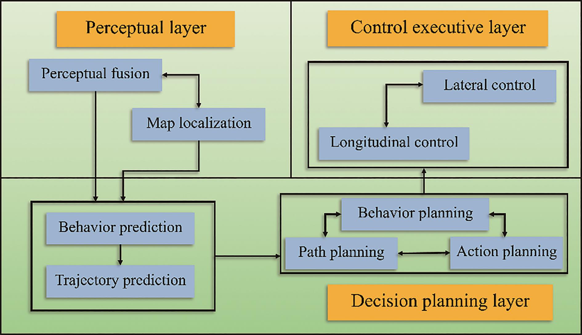
Figure 1. Hierarchical structure of the intelligent connected vehicle (ICV) system.
Decision planning of the ICV mainly refers to the planning and correction of the final driving path of the vehicle. Path planning, or global path planning, refers to the use of path planning algorithms to find the optimal path with the shortest travel distance or travel time from the starting point to the end point, given a map of the environment and the starting and ending locations. Behavior planning and action planning belong to local path planning, which refers to the consideration of vehicle kinematic constraints and comfort indexes, focusing on the consideration of the current completely unknown or partially knowable local environmental information of the vehicle, and making corrections to the global path so that the car has good obstacle avoidance capability. The above planning functions work together to enable ICVs to better plan the travel path from the start to the end point.
As already mentioned in the introduction, GPP based on topological maps is applicable when ICVs autonomously perform long-distance, multi-location driving assignments. When the ICV performs such driving tasks, which involve starting from a starting point, passing through certain designated locations to pick up or distribute goods, and finally reaching the destination, GPP can be abstracted to solve such a special TSP, i.e., the fixed open TSP. Before doing so, it is necessary to analyze the ICV's travel time.
2.2. Vehicle Travel Time Analysis
The driving speed of ICVs is affected by weather conditions and time periods. In order to accurately describe the spatial-temporal characteristics of ICVs driving, a model of ICVs speed characteristics under different weather conditions and time periods was established based on the actual monitoring data of the project platform (China Automotive Technology Research Center - China Automotive Condition Information System Platform), as shown in Figure 2.
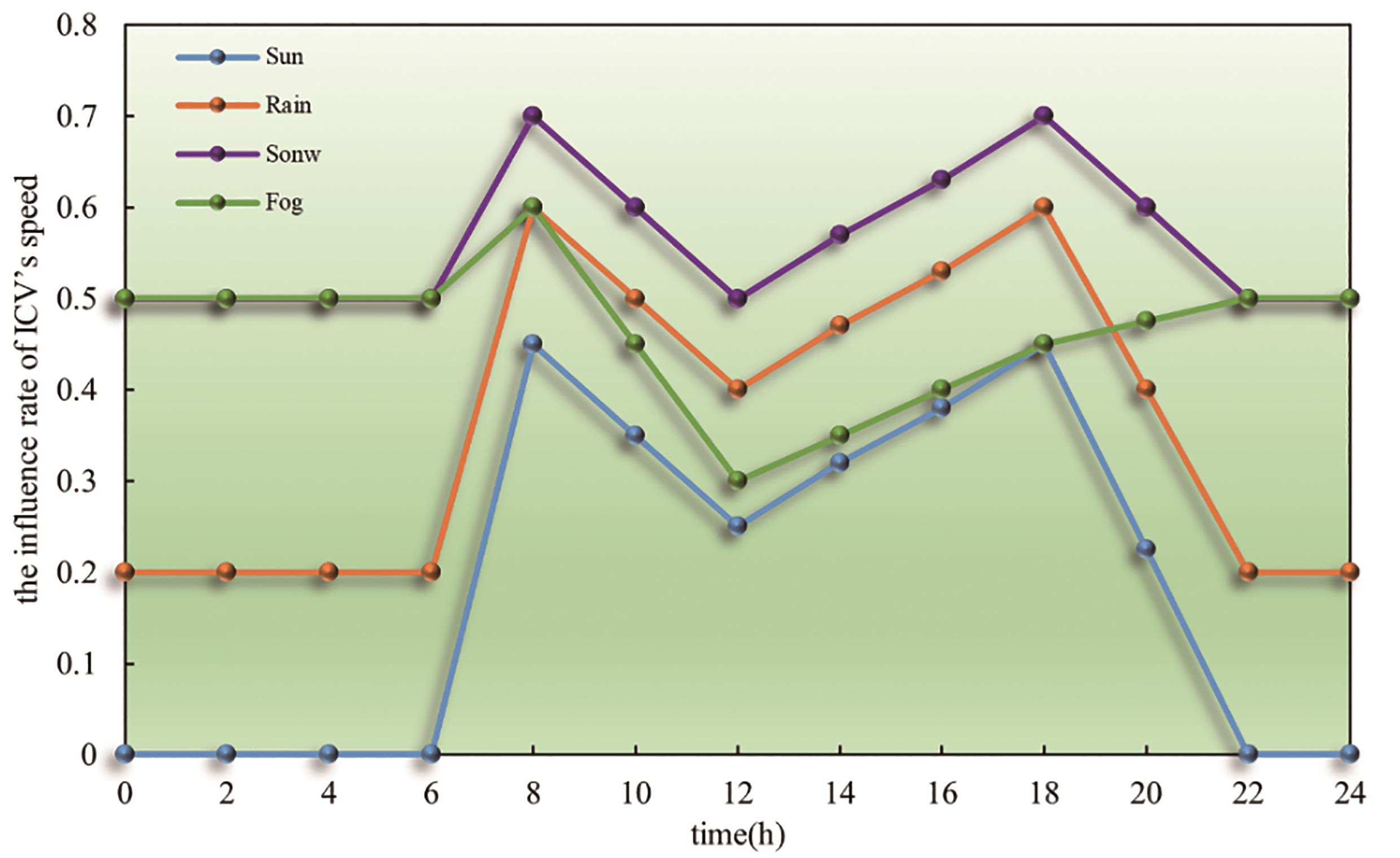
Figure 2. The influence rate of ICV’s speed.
Therefore,  ,the travel speed of ICV from city Vi to city Vj in planning path, can be expressed as:

where  denotes the distance from city Vi to city Vj in planning path,
  represents the traveling speed of ICV, which can be defined by the following formula:
![]()
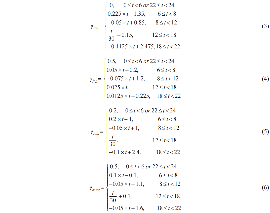
where,  is the average driving speed of ICV, and
  (con = sun, fog, rain, sown) is the speed influence rate of ICV, and depending on the weather and time period when driving, it takes the following rules:
2.3. The Fixed Open Travelling Salesman Problem (TSP)
The TSP is a classical combinatorial optimization task. From a graph-theoretic point of view, the task is essentially to find a Hamiltonian loop with minimum weights in a weighted completely undirected graph. Since the feasible solution of this task is the full permutation of all vertices, it is an NP-complete task that generates combinatorial explosion as the number of vertices increases. Because of its wide application in the fields of transportation, circuit board design and logistics distribution, scholars at home and abroad have conducted a lot of research on it [18,19].
The mathematical model of classical TSP can be described as follows: the location information of n cities or the distances between cities are known, and a traveler visits each city once, and only once starting from a specific city and finally returning to the departure city. How to arrange the cities so that the distance traveled by the traveler is the shortest? In short, the objective is to find a shortest path that traverses n cities, or search for a natural subset X = {1, 2, ∙∙∙, n} (The elements of X denote the numbering of the n cities) of an arrangement π(X) = {V1, V2, ∙∙∙, Vn} such that:

takes the minimum value, where d (Vi, Vi+1) denotes the distance from city Vi to city Vi+1 in planning path.
Currently, the TSP has been extended in various forms, such as the multiple-visit TSP (MVTSP) [20], the TSP with pickup and delivery (TSPPD), and the multi-person TSP (MTSP) [21], and when both TSPPD and MTSP are considered, TSP is transformed into a vehicle routing problem (VRP).
When a ICV performs a long-distance, multi-location driving assignment, this process can be considered as a TSP, i.e., the origin and the target city are known, and an optimal path with the shortest distance is planned so that the ICV reaches the target city after visiting each city node and does not need to return to the origin. The TSP overview diagram is shown in Figure 3.
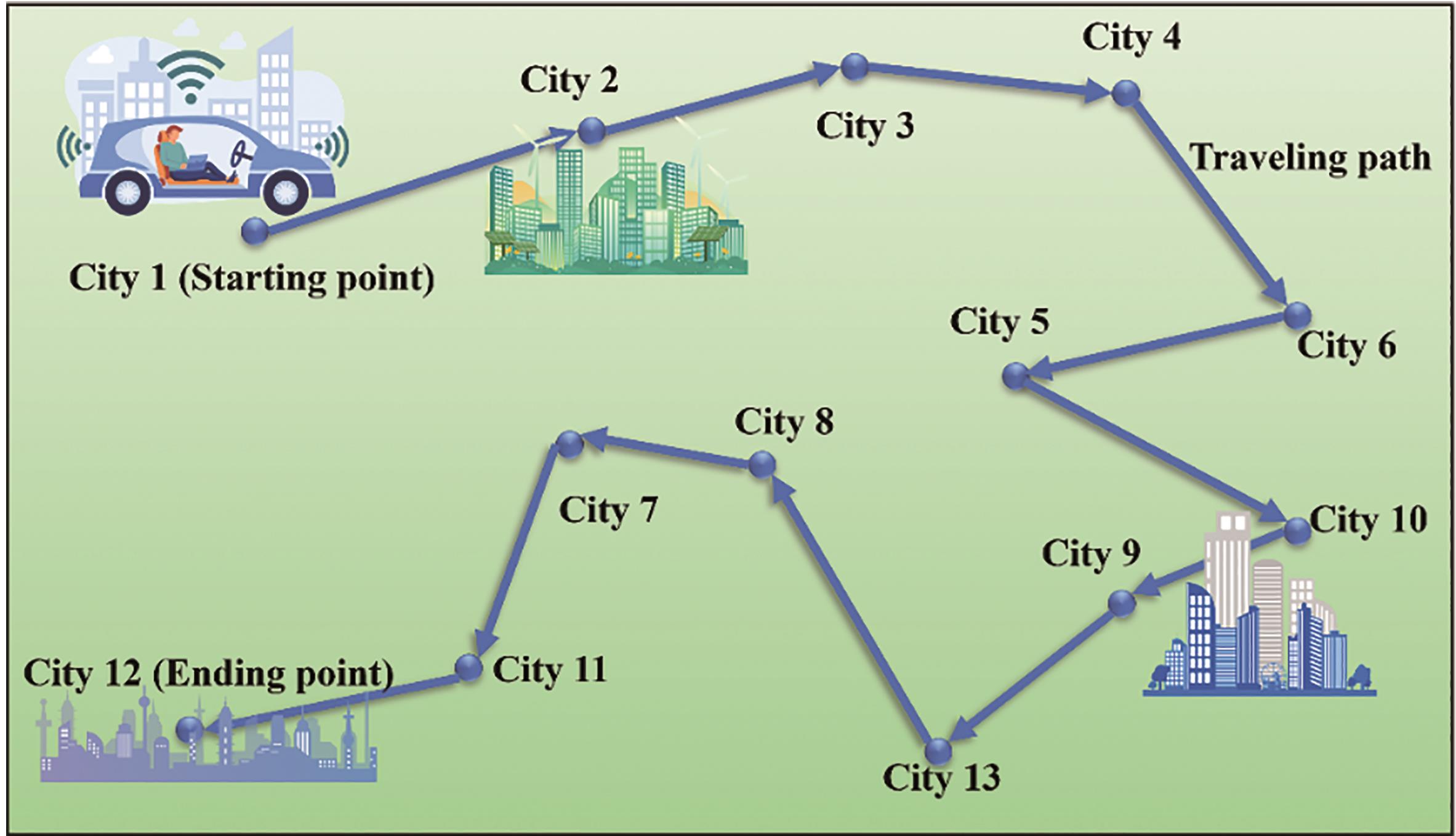
Figure 3. Overview diagram of the fixed open travelling salesman problem (TSP).
The mathematical model is: let the departure point be Vs and the target city be Ve, search for a natural subset X = {0,1, ∙∙∙, n+1} (The elements of X denote the numbering of the n+2 cities) of an arrangement π(X) = {Vs, Vj, ∙∙∙, Ve}, j = (1, 2, ∙∙∙, n), such that:

takes the minimum value. In conjunction with subsection 2.2, the following expression can be obtained:

2.4. Model Establishment
According to the above analysis, the TSP is established as a model of multi-objective optimization:
For city i and city j, let the set of path cities be C = {1, 2, ∙∙∙, n}and the set of all cities is N = C ∪ {0, n+1}, and then C’ = {1, 2, ∙∙∙, n+1}. Let dij represent the distance of the ICV from city i to city j, tij represents the travel time of the ICV from city i to j, and the travel cost per unit time of the ICV is cv, if the decision variable is set

The objective function (optimal value) is shown in Equation (10):

Constraints are shown in Equations (11) to (14):
Each city (except the starting point) must be visited once:

Every city that is visited must be set being visited once by other cities, but the starting point can only be set for visiting other cities, and the end point can only be visited:

The starting point has at most one exit arc and cannot be directly connected to the end point:

Ensure that no subloops exist in the planned path:

2.5. Planning Algorithms
Genetic algorithm (GA) is a search method that mimics the natural evolutionary process by simulating the Darwinian evolutionary theory of "natural selection" and the biological evolutionary process of genetics [22]. In order to ensure the ideal search effect for the path distance minimization task, the article combines the idea of simulated annealing and constructs a genetic-annealing algorithm (GAA), the main components of which are described below.
Population initialization: The initial population is the set of partial feasible solutions of the optimization problem. Assuming that the population size is L, the initial population P0 is denoted as P0 = {I1, I2, ∙∙∙, IL}, where Iμ = {Vs, Vj, ∙∙∙, Ve}, μ = (1, 2, ∙∙∙, L) denotes the μ-th feasible solution, in which the algorithm calls "the μ-th individual".
Adaptation calculation: Adaptation is used to evaluate the ability of an individual to adapt to its environment and plays a crucial role in the evolutionary process of an individual. A high fitness value indicates that the individual is superior and has a high probability of survival. On the contrary, it is difficult to survive with low fitness value. Combined with simulated annealing, the fitness function Fμ is constructed:

where Fμ denotes the fitness value of the μ-th individual, f(μ) is the value of the optimization objective function of the μ-th individual, W(g) denotes the annealing temperature function, which is related to the population generation g, w0 denotes the initial annealing temperature (usually w0 = 2gmax), and gmax denotes the maximum evolutionary generation of the population, aw is the annealing temperature coefficient, which usually takes a value slightly lower than 1. The fitness function proposed in this chapter can be adjusted adaptively as the population evolves. In the early stages of algorithm evolution, the difference in fitness between individuals in the population is large, which will help the algorithm to select individuals with higher fitness for crossover and variation operations. As the number of generations of population evolution increases, the difference in fitness between individuals in the same generation gradually decreases, which will help increase the ability of the algorithm to find local advantages.
3. Simulation Results and Analysis
3.1. Sample Analysis
In order to simulate the GPP task of driving a smart connected car to visit multiple cities or locations, we randomly generated 50 city coordinates in Matlab, and the coordinate statistics of some cities are shown in Table 1. Among them, the starting city number is 1 and the ending city number is 37. The location coordinates of the cities and the distance between the cities are shown in the Figure 4.
Table 1. Coordinates of some cities.
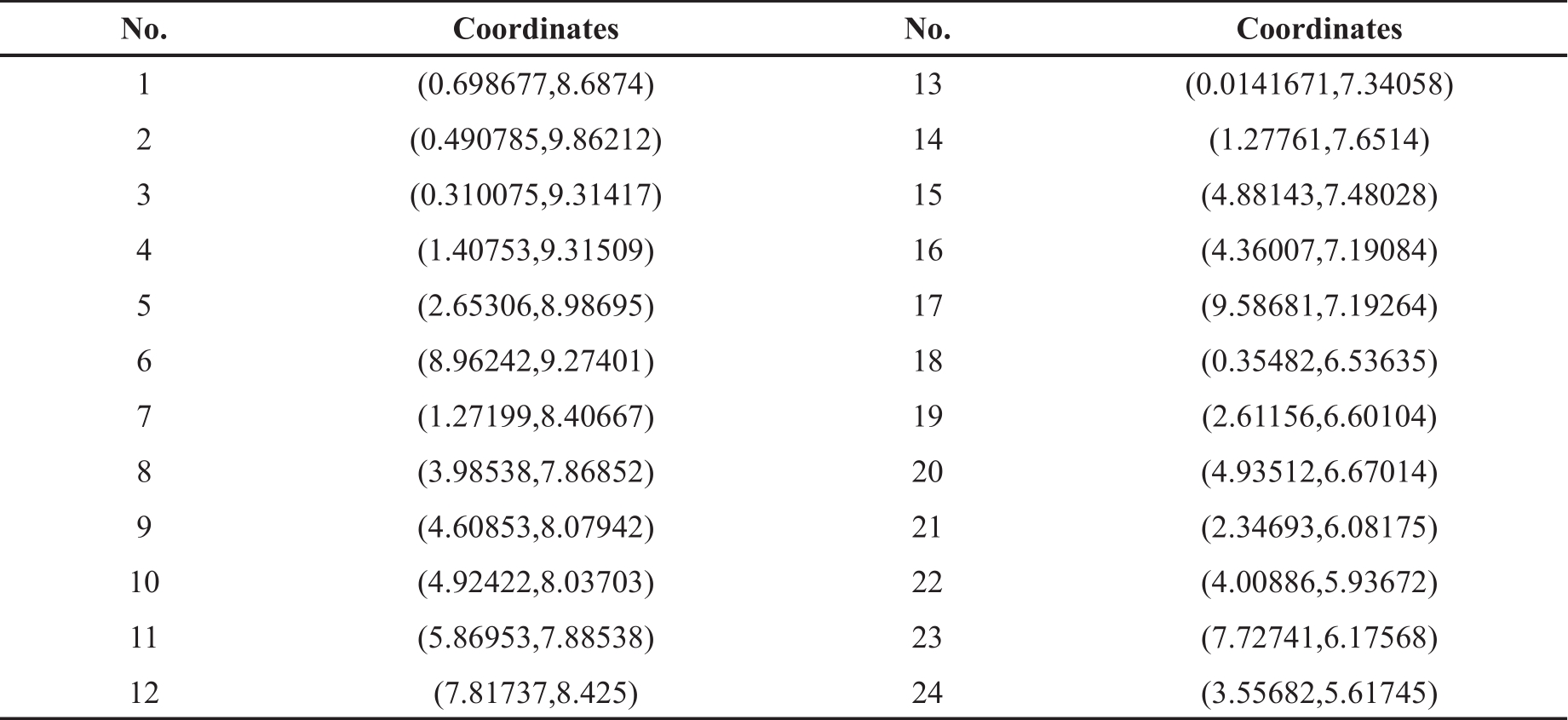
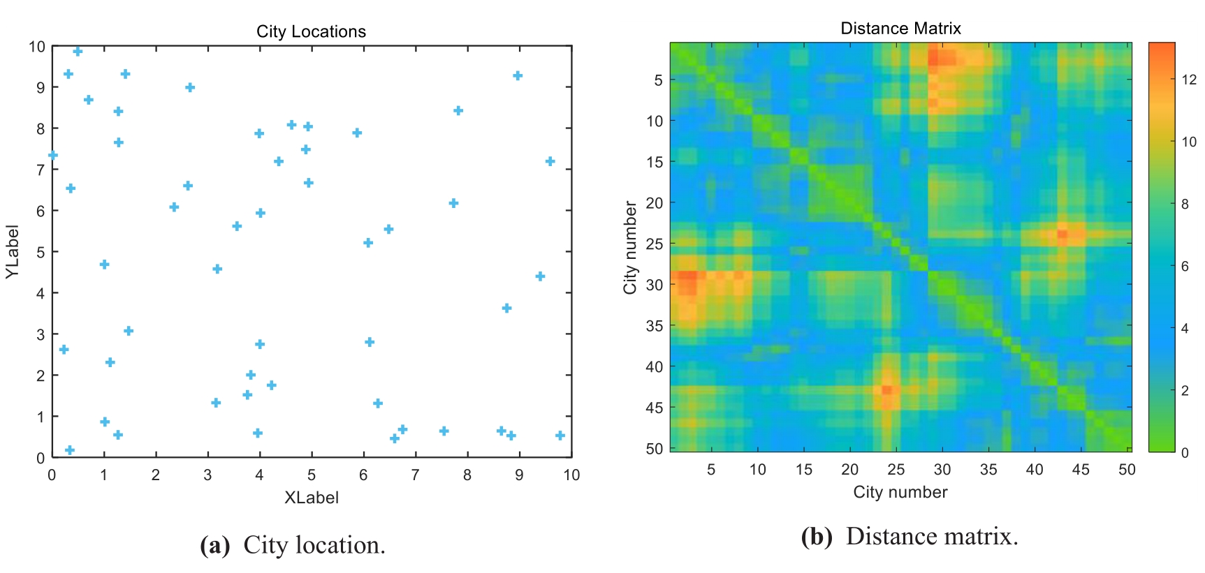
Figure 4. City data situation.
In order to test the performance of GAA, we chose GA, ACA and GAA for simulation respectively, and the initialization parameters of the three algorithms were set as follows:
GA: The initial population size L was 100, iteration number gmax was set to 103, proportion of retained individuals after selection (generation gap) was 0.25.
ACA: The maximum number of iterations NCmax, for the purpose of algorithm comparison, was also selected in this paper as 103; the number of ants m, generally set as 1.5 times the number of cities, α took the value of 1, β takes the value of 5, the volatility constant of pheromones on the path ρ took the value of 0.1.
GAA: The initial population size L was 100; iteration number gmax was set to 103, aw = 0.95, proportion of retained individuals after selection (generation gap) was 0.25.
Simulation environment: Windows 11, Intel i5-12500H, and 16GB RAM. Simulation platform: Matlab2022a.
3.2. Simulation Results
(1) Firstly, we optimized the performance of the three algorithms when the weather conditions were sunny and the ICV was driven only at night (22:00 PM to 6:00 AM). The values of the average driving speed and the travel cost per unit time cv were both set to 1 unit, and the crossing or service time while passing through each city was set to 0.5 units. The optimal one-time results of the three algorithms for multiple runs on the computer were as follows:
The optimal solution of the objective function (total cost) of ACA was 87.9904 units with a running time of 7.363592 seconds and the optimal travel path was: 1–7–14–18–13–3–2–4–5–8–16–15–9–10–11–12–6–17–23–25–26–33–40–47–44–45–46–48–49–30–29–20–22–24–28–21–19–27–31–35–34–41–42–50–39–38–36–32–43–37. The travel path is shown in Figure 5a.
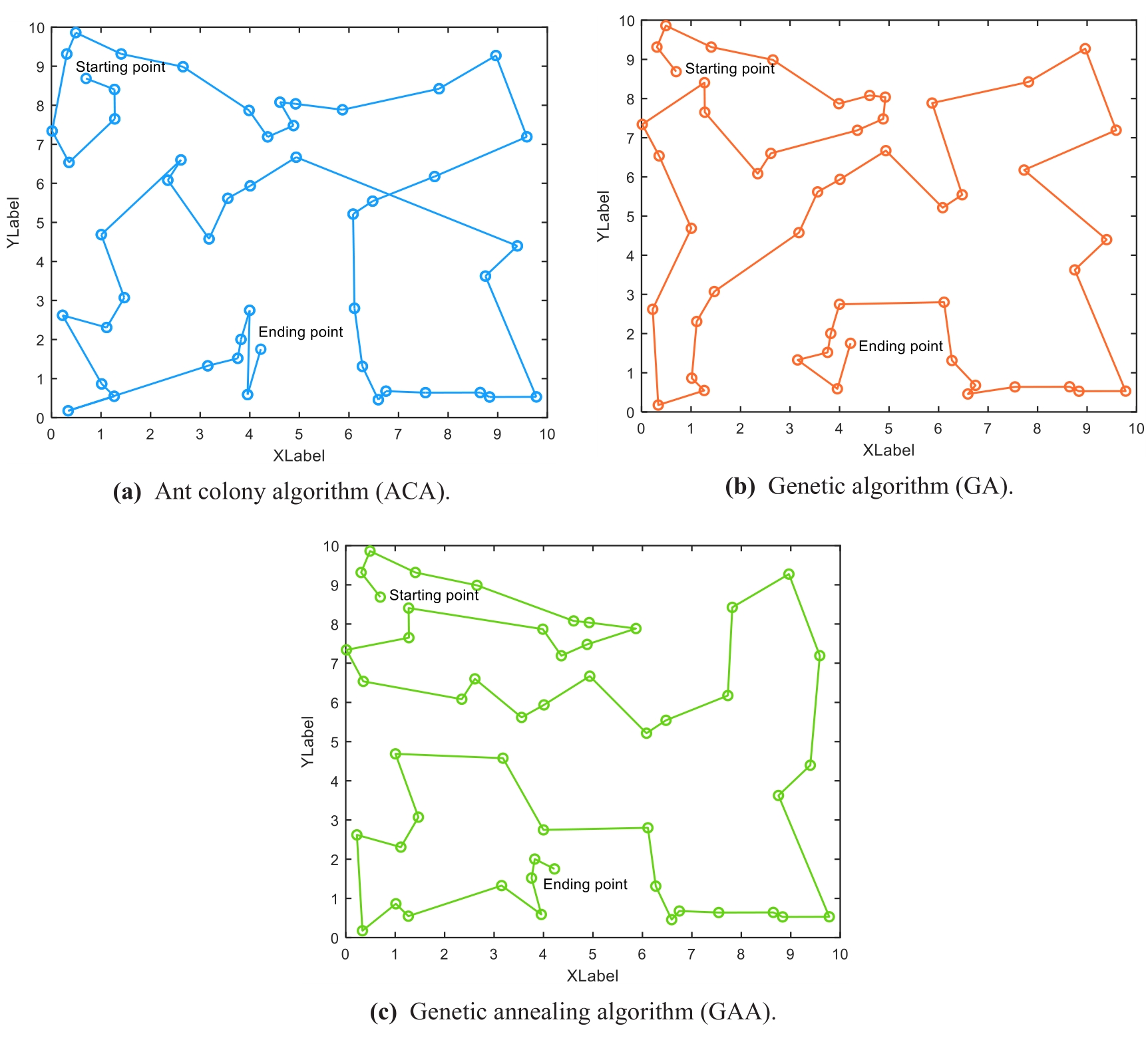
Figure 5. Optimal paths for three algorithms for night driving.
The optimal solution of the objective function (total cost) of GA was 85.8883 units with a running time of 2.983524 seconds and the optimal travel path was: 1–3–2–4–5–8–9–10–15–16–19–21–14–7–13–18–27–34–50–42–41–35–31–28–24–22–20–26–25–11–12–6–17–23–29–30–49–48–46–45–47–44–40–33–32–36–38–39–43–37. The travel path is shown in Figure 5b.
The optimal solution of the objective function (total cost) of GAA was 82.0111 units with a running time of 2.566709 seconds and the optimal travel path was: 1–3–2–4–5–9–10–11–15–16–8–7–14–13–18–21–19–24–22–20–26–25–23–12–6–17–29–30–49–48–46–45–44–47–40–33–32–28–27–31–35–34–50–41–42–39–43–38–36–37. The travel path is shown in Figure 5c.
Among them, we recorded the iterative process and running time of the three algorithms as a way to compare the performance of the three algorithms. The optimization iteration chart and running time comparison are shown in Figure 6.
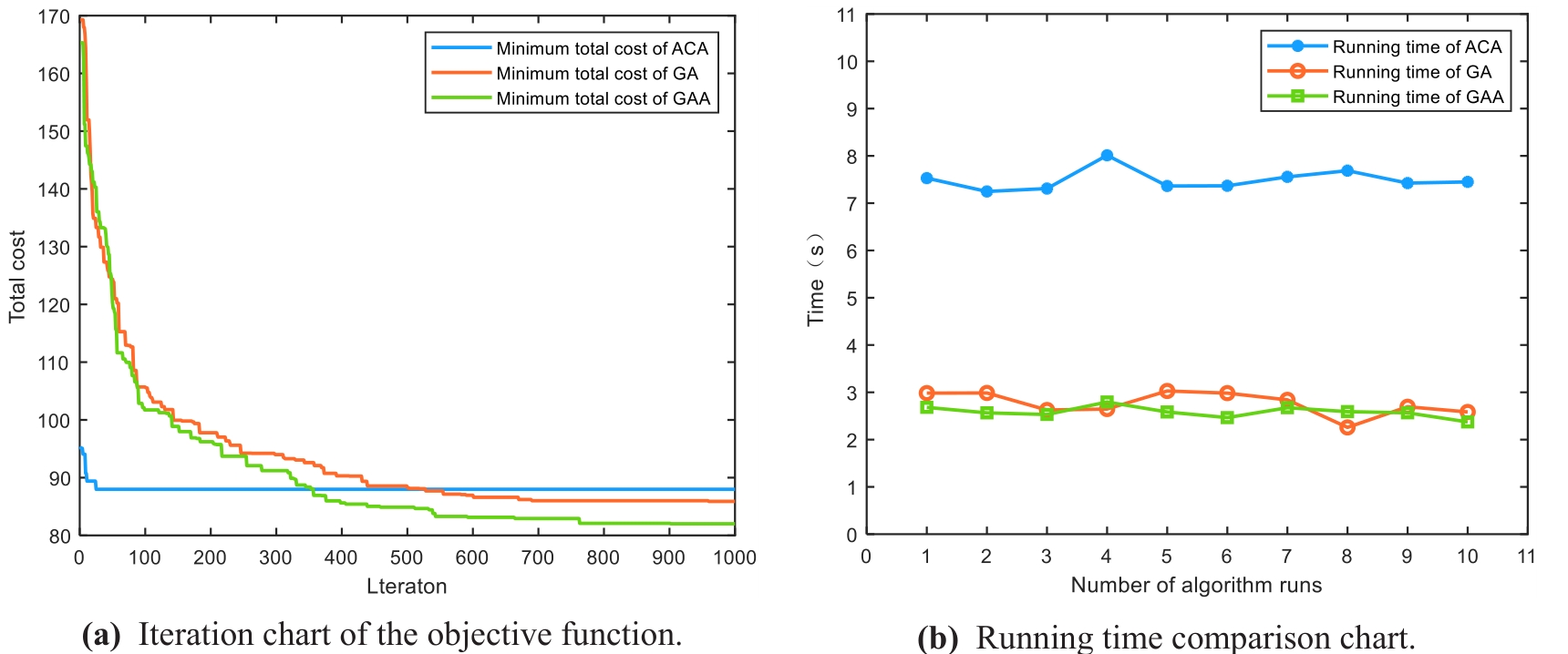
Figure 6. Algorithm Performance Comparison.
(2) Finally, the performance of the three algorithms was optimized when the weather conditions were sunny and the ICVs were driven only during daytime (6:00 AM to 22:00 PM). Other parameter settings were the same as the first group of experiments. The optimal one-time results of the three algorithms for multiple runs on the computer were as follows:
The optimal solution of the objective function (total cost) of ACA was 123.6004 units with a running time of 7.501107 seconds and the optimal travel path was: 1–7–14–18–13–3–2–4–5–8–16–15–10–9–11–12–6–17–23–25–26–20–22–24–28–21–19–27–31–35–34–41–42–50–39–38–36–32–33–40–44–47–45–46–48–49–30–29–43–37. The travel path is shown in Figure 7a.
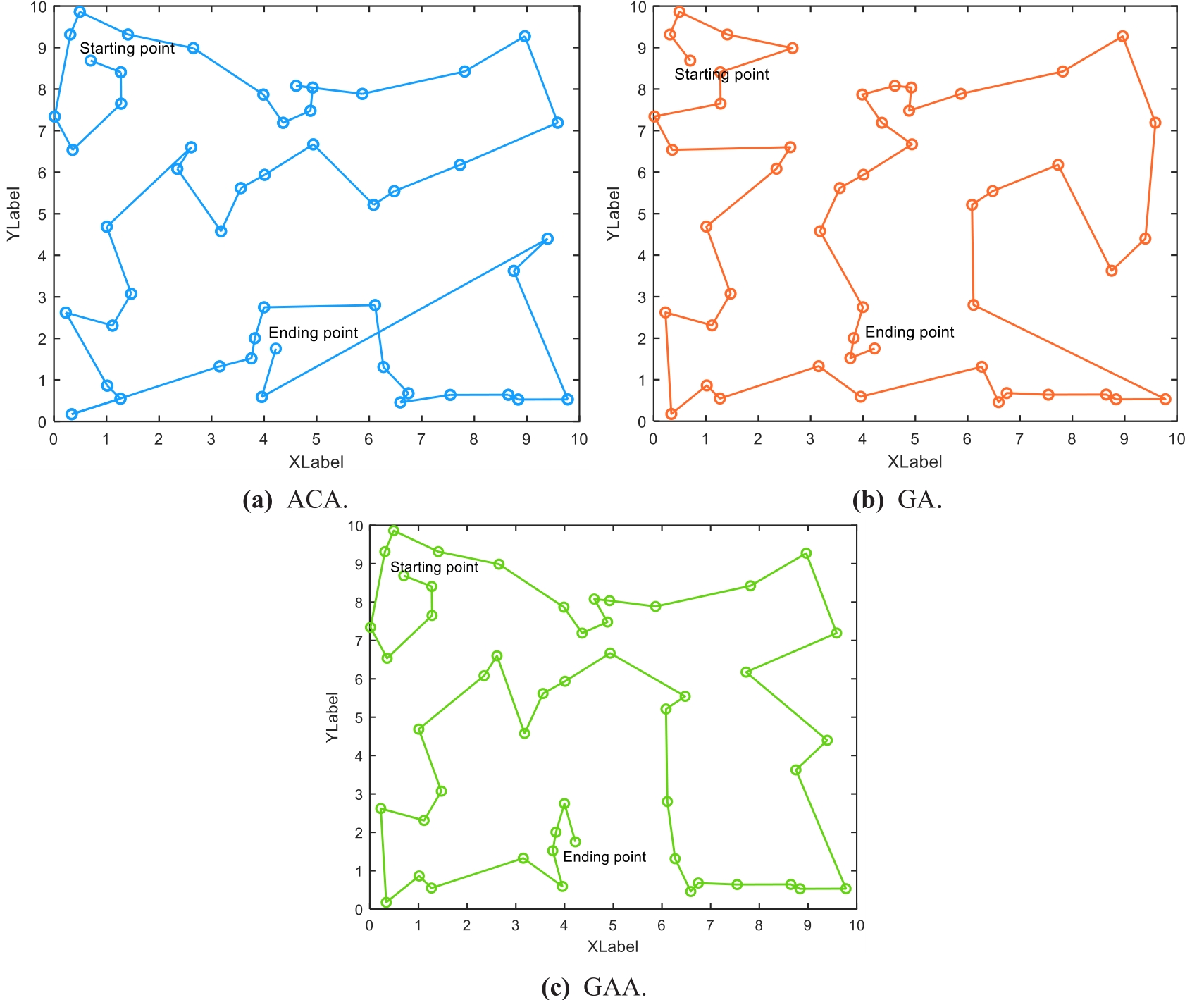
Figure 7. Optimal paths for the three algorithms for daytime driving.
The optimal solution of the objective function (total cost) of GA was 112.3162 units with a running time of 3.065543 seconds and the optimal travel path was: 1–3–2–4–5–7–14–13–18–19–21–27–131–35–34–50–41–42–39–43–40–47–44–45–46–48–49–33–26–25–23–30–29–17–6–12–411–15–10–9–8–16–20–22–24–28–32–36–38–37. The travel path is shown in Figure 7b.
The optimal solution of the objective function (total cost) of GAA was 105.8266 units with a running time of 2.870923 seconds and the optimal travel path was: 1–7–14–18–13–3–2–4–5–8–16–15–9–10–11–12–6–17–23–29–30–49–48–46–45–44–47–40–33–26–25–20–22–24–28–19–21–27–31–35–334–50–41–42–39–43–38–36–32–37. The travel path is shown in Figure 7c.
Similarly, we recorded the iterative process and running time of the three algorithms as a way to compare the performance of the three algorithms. When comparing the running times, it was noticed that ACA usually found the optimal solution quickly within 200 to 400 generations. After reaching that point, it no longer optimized, and subsequent iterations may result in the waste of time. Therefore, we reduced the NCmax of ACA to 400 generations and then ran it 10 times for the running time comparison, and GA and GAA remained at 103 generations. The comparison of optimization iteration graph and running time is shown in Figure 8.
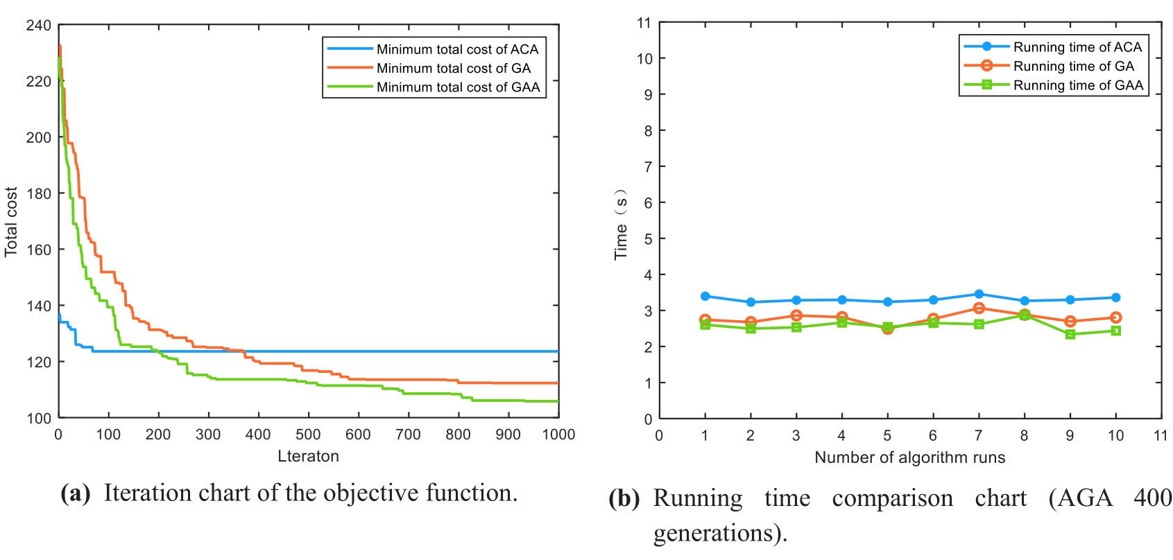
Figure 8. Algorithm Performance Comparison.
3.3. Analysis of Results
Firstly, from the optimization results, all three algorithms have shown good optimization effects on fixed open TSP, but the optimal solution value found by GAA was smaller than GA and ACA. Additionally, ACA could find the optimal solution quickly, but it had the largest optimal solution value. Secondly, from the iterative process, ACA basically found the optimal solution in approximately 200 to 400 generations, while GA and GAA needed around 1000 generations to find the optimal solution. Finally, in terms of running time, after the introduction of the new fitness function, the complexity of GAA did not improve compared to the traditional genetic algorithm, and the optimization search time was similar to that of GA. When the number of iterations was the same, the running time of ACA was much larger than that of GA and GAA. When the number of iterations of ACA was adjusted to a suitable value, the running time of the algorithm was still slightly higher than that of GA and GAA. In conclusion, among the three algorithms, GAA could better perform the GPP and optimization tasks of ICVs when driving over long distances and multiple locations.
4. Conclusion
In this paper, a non-closed-loop traveling salesman problem (TSP) model with fixed starting and ending points was constructed for topological map-based GPP for long-distance and multi-location assignments of ICVs, combined with analysis of the travel times of ICVs. To solve this mathematical model, an improved genetic algorithm was proposed. Furthermore, we simulated and optimized the global path planning of ICVs under road and weather conditions for both daytime and nighttime driving. We utilized ACA, GA and GAA, respectively, to verify the effectiveness of the three algorithms in completing such tasks. Based on the optimization processes and results, the proposed GAA outperformed the traditional topological map-based de-global path planning optimization algorithm in facing this task. The future work to be further investigated would continue to extend the topological map-based ICV’s global path planning model and algorithm.
Author Contributions: Conceptualization, H.W. and S.C.; methodology, H.W.; software, X.Y.; validation, S.C. and X.Y.; formal analysis, S.C.; investigation, Z.W.; resources, Z.L.; data curation, X.Y.; writing—original draft preparation, S.C.; writing—review and editing, H. W.; visualization, S. C.; supervision, Z. L.; project administration, Z. W.; funding acquisition, H.W. All authors have read and agreed to the published version of the manuscript.
Funding: This research was funded by the Training Plan for Young Backbone Teachers in Colleges and Universities of Henan Province, grant number 2021GGJS032.
Data Availability: Statement: The date that support the findings of this study are available from the corresponding author upon reasonable request.
Conflicts of Interest: The authors declare no conflict of interest. The role of the funders in the design of the study: conceptualization and methodological in the writing of the manuscript and in the decision to publish the results.
References
- Zhuang, Z.; Guan, Y.; Xu, S.; et al. Reconfigurability in Automobiles—Structure, Manufacturing and Algorithm for Automobiles. International Journal of Automotive Manufacturing and Materials 2022, 1(1), 1. DOI: https://doi.org/10.53941/ijamm0101001
- Liu, H.; Saksham, D.; Shen, M.; et al. Industry 4.0 in Metal Forming Industry Towards Automotive Applications: A Review. International Journal of Automotive Manufacturing and Materials 2022, 1(1), 2. DOI: https://doi.org/10.53941/ijamm0101002
- Wang, B.; Han, Y.; Wang, S.; et al. A Review of Intelligent Connected Vehicle Cooperative Driving Development.Mathematics 2022, 10(19), 3635–3635. DOI: https://doi.org/10.3390/math10193635
- Wang, H.; Li, G.; Hou, J.; et al. A Path Planning Method for Underground Intelligent Vehicles Based on an Improved RRT* Algorithm. Electronics 2022, 11(3), 294–294. DOI: https://doi.org/10.3390/electronics11030294
- Li, H.; Zhao, T.; Dian S. Forward search optimization and subgoal-based hybrid path planning to shorten and smooth global path for mobile robots. Knowledge-Based Systems 2022, 258, 110034. DOI: https://doi.org/10.1016/j.knosys.2022.110034
- Daddi, G.; Notaristefano, N.; Stesina, F.; et al. Assessing an Image-to-Image Approach to Global Path Planning for a Planetary Exploration. Aerospace 2022, 9(11), 721–721. DOI: https://doi.org/10.3390/aerospace9110721
- Yang, X.; Shi, Y.; Liu, W.; et al. Global path planning algorithm based on double DQN for multi-tasks amphibious unmanned surface vehicle. Ocean Engineering 2022, 266, 112809. DOI: https://doi.org/10.1016/j.oceaneng.2022.112809
- Luo, M.; Hou, X.; Yang J. Surface Optimal Path Planning Using an Extended Dijkstra Algorithm. IEEE ACCESS 2020, 8, 147827–147838. DOI: https://doi.org/10.1109/ACCESS.2020.3015976
- Wang, H.; Lou, S.; Jing, J.; et al. The EBS-A* algorithm: An improved A* algorithm for path planning. PloS one 2022, 17(2), e0263841. DOI: https://doi.org/10.1371/journal.pone.0263841
- Wu, Y.; Li, Z.; Sun, C.; et al. Measurement and control of system resilience recovery by path planning based on improved genetic algorithm. Measurement and Control 2021, 54(7–8), 1157–1173. DOI: https://doi.org/10.1177/00202940211016094
- Wu, C.; Zhou, S.; Xiao L. Dynamic Path Planning Based on Improved Ant Colony Algorithm in Traffic Congestion. IEEE Access 2020, 8, 180773–180783. DOI: https://doi.org/10.1109/ACCESS.2020.3028467
- Niu, C.; Li, A.; Huang, X.; et al. Research on Global Dynamic Path Planning Method Based on Improved Algorithm. Mathematical Problems in Engineering 2021, 2021, 1–13. DOI: https://doi.org/10.1155/2021/4977041
- Zhao, J.; Ma, X.; Yang, B.; et al. Global path planning of unmanned vehicle based on fusion of A* algorithm and Voronoi field. Journal of Intelligent and Connected Vehicles 2022, 5(3), 250–259. DOI: https://doi.org/10.1108/JICV-01-2022-0001
- Hua, C.; Niu, R.; Yu, B.; et al. A Global Path Planning Method for Unmanned Ground Vehicles in Off-Road Environments Based on Mobility Prediction. Machines 2022, 10(5), 375. DOI: https://doi.org/10.3390/machines10050375
- Liu, L.S.; Lin, J.F.; Yao, J.X.; et al. Path Planning for Smart Car Based on Dijkstra Algorithm and Dynamic Window Approach. Wireless Communications and Mobile Computing 2021, 2021, 1–12. DOI: https://doi.org/10.1155/2021/8881684
- Yuan, Z.; Yang, Z.; Lv, L.; et al. A Bi-Level Path Planning Algorithm for Multi-AGV Routing Problem. Electronics 2020, 9, 1351. DOI: https://doi.org/10.3390/electronics9091351
- Zhou, Q.; Li, J.; Xu H. Artificial Intelligence and Its Roles in the R&D of Vehicle Powertrain Products. International Journal of Automotive Manufacturing and Materials 2022, 1(1), 6. DOI: https://doi.org/10.53941/ijamm0101006
- Traub, V.; Vygen, J.; Zenklusen R. Reducing Path TSP to TSP. Siam Journal on Computing 2021, 51(3), 24–53. DOI: https://doi.org/10.1137/20M135594X
- Hu, Y.; Duan Q. Solving the TSP by the AALHNN algorithm. Mathematical Biosciences and Engineering 2022, 19 (4), 3427–3448. DOI: https://doi.org/10.3934/mbe.2022158
- Kowalik Ł.; Li, S.; Nadara, W.; et al. Many-visits TSP revisited. Journal of Computer and System Sciences 2022, 124, 112–128. DOI: https://doi.org/10.1016/j.jcss.2021.09.007
- Tong, J.; Qiu, Z.; Zhou, H.; et al. Optimizing the path of seedling transplanting with multi-end effectors by using an improved greedy annealing algorithm. Computers and Electronics in Agriculture 2022, 201, 107276. DOI: https://doi.org/10.1016/j.compag.2022.107276
- Razali, M. R.; Faudzi, A. A. M.; Shamsudin, A. U.; et al. A hybrid controller method with genetic algorithm optimization to measure position and angular for mobile robot motion control. Frontiers in Robotics and AI 2023, 9, 1087371. DOI: https://doi.org/10.3389/frobt.2022.1087371