

Downloads
Download


This work is licensed under a Creative Commons Attribution 4.0 International License.
Article
Research and Analysis on Motion Planning Method of Intelligent Connected Vehicles
Heng Wang 1,2, Xianyi Yang 1,2, Zhengbai Liu 3, and Zhenfeng Wang 1,2, *
1 College of Mechanical and Electrical Engineering, Henan Agricultural University, Zhengzhou 450002, China
2 Henan Provincial Cold Chain Information and Equipment Laboratory for Logistics of Agricultural Products, Zhengzhou 450002, China
3 School of Innovation and Entrepreneurship, Southern University of Science and Technology, Shenzhen 518055, China
* Correspondence: zfking@henau.edu.cn
Received: 23 September 2022
Accepted: 21 November 2022
Published: 18 December 2022
Abstract: Combined with the tire model, a two-degree-of-freedom model is proposed in this study. At the same time, a turning control model is analyzed, which lays the foundation for the subsequent local path planning, that is, the simulation control of lane changing and obstacle avoidance. The co-simulation of CarSim and Simulink is used to realize the tracking control of trajectories, and the given reference trajectory can be tracked with high precision in the serpentine rod penetration test, so as to verify the stability of the control algorithm control. A set of optimal trajectories of straight lane change and curved lane change are selected as the reference trajectories of the controller, and the target speed of the lane change is given in the CarSim speed control module. The simulation results show that the motion planning error is extremely small that completes the high-precision automatic control of steering, and this helps realize the tracking of a given trajectory, reflecting the good trackability of the planned lane-changing trajectory from the side. Aiming at the automatic lane changing process of the intelligent connected vehicle on different straight roads and curved roads, the V2V method is used to obtain the status information of the surrounding traffic vehicles where the multi-objective optimization method is used to determine the optimal trajectory. Driving with reference to the trajectory realizes the coordination and unity of planning and control.
Keywords:
intelligent connected vehicles motion planning kinematic model dynamic model1.Introduction
With the increasing number of automobiles on the road, a series of problems caused by automobiles, such as traffic jams, traffic accidents and exhaust emissions, are becoming more and more obvious [1]. People are no longer satisfied with the basic functions of automobiles. The demand for intelligent automobiles is getting higher and higher, leading the automotive industry to face unprecedented challenges. Intelligent driving automobiles can reduce traffic accidents, improve vehicle safety, ease traffic congestion, reduce driving fatigue, reduce fuel consumption, and bring convenience to people’s daily automobile use [2,3]. Intelligent driving vehicles have attracted more and more attention in the field of automobile-related research and society, and are deemed to have broad application prospects.
At present, scholars from many countries in the world have conducted in-depth research on dynamic path planning [4‒6]. The local path planning method based on a specific function has the advantages of simple calculation, fast and smooth curvature, and has been widely used in vehicle lane changing and obstacle avoidance. Based on the dynamic model of the smart automobile, the smooth trajectory is generated by the sixth-order polynomial, and the dynamic path planning of the smart automobile in an unknown environment is realized through the rolling window optimization strategy [7]. For safety driving, the generated trajectory is relatively smooth, which ensures the steering stability of the vehicle during driving. In order to improve the maneuvering stability during active obstacle avoidance and lane changing, relevant scholars use the four-wheel independent steering technology to study the path planning algorithm [8]. Based on the four-wheel steering vehicle model, a seven-degree polynomial is used to design the path planning algorithm, which improves the ride comfort during obstacle avoidance and reduces the lane-changing impact [9]. Relevant scholars have proposed a real-time path planning method for obstacle avoidance of off-road autonomous vehicles [10]. A curvilinear coordinate system is generated according to the known road center points, and multiple cubic polynomial paths are generated as candidate paths. A candidate path is selected as the optimal path for consistency. In addition to polynomials, common functions in local path planning methods based on specific functions, trigonometric functions, arcs and trapezoidal acceleration trajectories are also used in local path planning [11,12]. In local path planning, different functions are basically the same. Relevant scholars use the grid method for local path planning, divide the drivable area of the vehicle into uniform grids, and conduct sampling regularly [13]. The information of the sampling points includes position information and heading angle information, and the sampling points are connected by spline curves [14]. However, due to the discretization of the heading angle, the trajectory planned by this method oscillates in the direction [15,16].
In order to track the lane changing trajectory, the model predictive control method is used to control the vehicle steering to complete the automatic lane changing. A three-degree-of-freedom vehicle model and a magic formula tire model are established, and the state space expression of the control system is obtained from the nonlinear dynamic model. According to the basic principle of model predictive control, the optimal control quantity of the system is obtained by predicting the equation and optimizing the solution process, and the design of the motion planning controller is completed. The co-simulation environment of CarSim and Simulink is built, and the simulation results show that the controller can realize the vehicle to complete the lane changing process accurately and smoothly on both straight and curved roads.
2.Method
2.1.Architecture of ICV
The intelligent connected vehicle (ICV) can realize information exchange and sharing between vehicles and intelligent terminals such as people, vehicles, roads and clouds. Generally, the ICV is capable of precepting complex environments, providing intelligent decision-making mechanisms, supplying collaborative control and offering execution functions, which can achieve safe, efficient, energy-saving and comfortable driving.
The intelligent connected vehicle control system is mainly composed of four parts: the environmental perception unit, the network communication unit, the autonomous decision-making unit and the underlying control unit. The relationship between the four functional units is shown in Figure 1. Here, the environmental perception unit and the network communication unit, respectively, obtains and transmits data to the autonomous decision-making unit; the autonomous decision-making unit feeds back control instructions to the network communication unit, and transmits the control instructions to the underlying control unit, and the underlying control unit performs specific operations in real time. Under certain conditions, the vehicle, road and environment form a complete system.
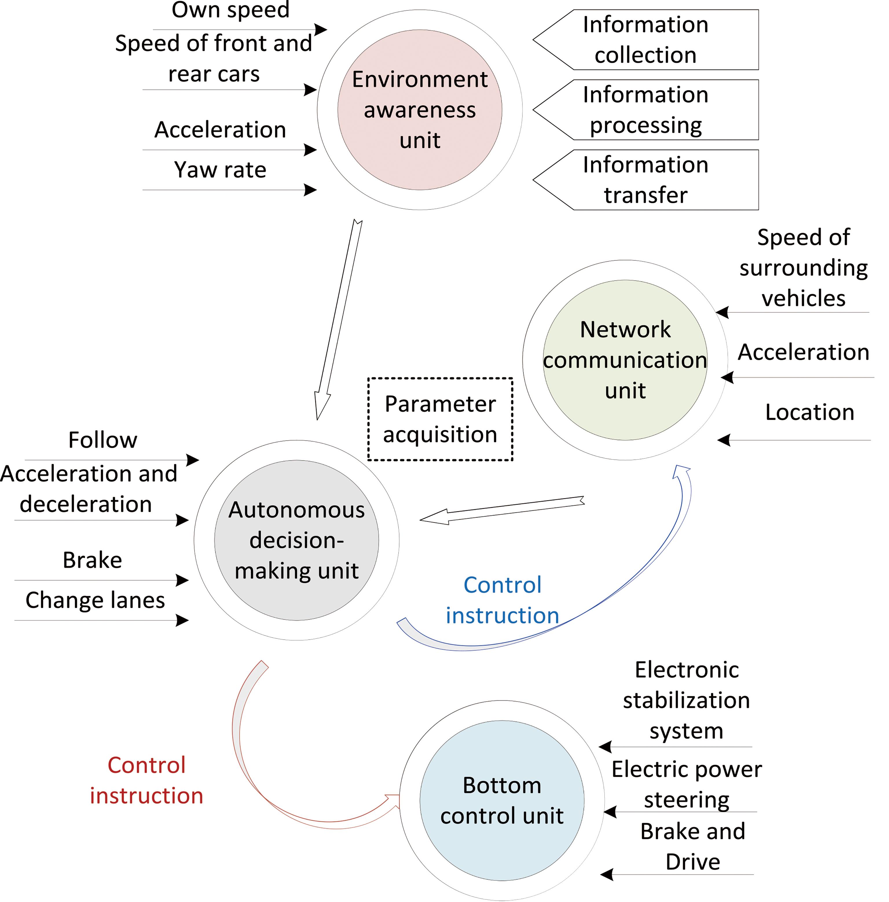
Figure 1. The composition of the intelligent connected vehicle system.
2.2.Calibration of Vehicle Modeling Coordinate System
For the international standard coordinate system in which the vehicle runs, the point O is the origin of the vehicle coordinate system and the center of mass of the vehicle, and it is assumed that no deviation occurs during the running of the vehicle. It is stipulated that the positive direction of the X-axis is the forward direction of the vehicle and is parallel to the ground. Pointing from the left side of the driver to the right is the positive direction of the Y-axis which is parallel to the ground. The planes are perpendicular to each other, and the downward direction is defined as the positive direction. This coordinate system satisfies the right-hand criterion. After the three axes of XYZ are determined, the translational motion along the respective axes and the rotation around each axis together constitute six degrees of freedom describing the operation of the vehicle, meanwhile multiple variables (including velocity, displacement, angular displacement and angular velocity) are defined to describe the motion.
2.3.Intelligent Vehicle Kinematics Model
In order to describe the laws of vehicle motion from a geometrical point of view, such as the changes in displacement and the speed of smart automobiles over time, we need to establish a corresponding kinematics model. Using the kinematic model, the planned trajectory can meet the geometric constraints, and the reliability of subsequent intelligent vehicle path tracking can thus be improved.
Mf is the axis of the front axle of the vehicle, and its coordinates are (Xf, Vf ), and Vf represents the center speed of the front axle when the vehicle is running; Mr is the axis of the rear axle of the vehicle, and its coordinates are (Xr, Vr ), and Vr represents the center speed of the rear axle when driving the vehicle. It is obvious that l is the wheelbase of the vehicle. The corresponding mathematical analysis of the kinematics model is as follows. The kinematic constraints of the front and rear axles of the vehicle are:
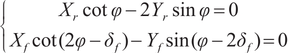
(1)
when the vehicle is running, the center speed Vr of the rear axle (Xr, Vr ) is:
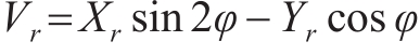
(2)
The front and rear wheels meet the following relationship:
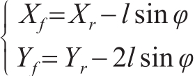
(3)
The yaw rate of the easy-to-obtain vehicle is:

(4)
The mathematical relationship of the vehicle kinematics model is:

(5)
When an obstacle or curve appears in the tracked path, it is avoided by the intelligent vehicle via steering the front wheels.
2.4.Modeling of Vehicle Dynamics
At present, there are three main types of commonly used tire models, namely the empirical tire model, semi-empirical tire model and classical theoretical tire model. In this study, the empirical tire model proposed by Pacjeka based on the magic formula is selected. The core of the magic formula is to use the trigonometric function formula to fit the tire test data, so as to obtain the longitudinal slip rate. The magic formula is as follows:

(6)
In the magic formula, the input is x, which is usually the longitudinal slip rate or the slip angle in the specific application of the tire model; the output is N, which is usually the lateral force Fc , longitudinal force Fl or return of the tire. The remaining coefficients B is the stiffness factor; C is the shape factor; D is the peak factor, which is related to the vertical load of the wheel and the camber angle; and E is the curvature factor.
Magic Formula tire models can be organized according to “input-X-output” to help understand and use. When the tire longitudinal slip rate and the tire slip angle are small, the tire is linear in both lateral and vertical directions, while the damping coefficient is constant.
The following assumptions are made when modeling:
(1) Set the driving environment as a plane and ignore the vertical jump of the vehicle;
(2) Set the tire to have only pure lateral deflection, and ignore the vertical and horizontal coupling of the vehicle tire force;
(3) The suspension is set as a rigid system, ignoring the motion of the suspension and the resulting coupling effects;
(4) Ignore the speed change rate when the vehicle is running, and ignore the transfer of the front and rear axle loads of the vehicle;
(5) Ignore the influence of horizontal and vertical aerodynamics;
This study adopts a two-degree-of-freedom vehicle model, ignoring both left and right movement of the load.
Combining the velocities Vx and Vy in the X-axis and Y-axis directions, the lateral and longitudinal velocities can be expressed as:

(7)
2.5.Front Wheel Rotation Angle Constraints of Intelligent Vehicles
In the actual turning process of the vehicle, if the steering angle is too large, the vehicle is in danger of side slipping and rollover. According to existing research results and experience, when the lateral acceleration of the vehicle is greater than 0.36 g, the tire cornering characteristics show significant nonlinearity, and this requires that the lateral acceleration of the intelligent vehicle should not be greater than 0.36 g when controlling the steering operation. In order to guarantee that the front wheel angle of the intelligent vehicle meets the requirements of ride comfort and safety at the same time, the influence of the turning radius of the vehicle speed should be taken into account, and this requires the front wheel angle to meet the following condition:
(8)
2.6.Model Predictive Control
The model predictive control (MPC) method models the system and solves the optimal control sequence. Basically, MPC consists of three parts: prediction model, feedback correction and rolling optimization. The prediction model predicts the future output value of the system through the input of the current time of the system and the historical information of the past time. The function of feedback correction corrects the ideal predictive value of the predictive model output, taking into account the nonlinearity, interference and other uncertainties of the real process. Rolling optimization is a rolling finite time domain optimization strategy, which determines the future control effect by optimizing the selected performance index.
In trajectory tracking, the system is modeled as a discrete state space equation:
(9)
According to the state equation, the recursive formula can be expressed as

(10)
According to the induction, the state quantity in the prediction time domain is calculated by:
(11)

(12)
The states in the prediction time domain are linear combinations of initial states and control variables. The loss function is composed of penalty terms of control quantity and error quantity.

(13)
where Q and R are constant matrices. Since x n is a linear combination of u , the loss function J is a quadratic function with respect to the control sequence u .
3.Simulation Results and Analysis
3.1.MPC Control System Co-simulated by Carsim and Simulink
The co-simulation method of CarSim and Simulink are employed to realize the control system. The CarSim software provides a high-precision vehicle model and a modeling environment for lane changing scenarios, while the Simulink platform provides the modeling of the control system, and data transfer is achieved through the interface between the two.
The vehicle and road modeling in the “human-vehicle-road” closed-loop system is completed in CarSim. For the study of the automatic lane changing process of intelligent connected vehicles, the “people” who make decisions and perform lane changing steering operations cannot use the driver preview model in CarSim, and must be replaced by an external control system. Simulink can realize complex control logic relationship, so we use Matlab/Simulink to complete the design of MPC control system. In Simulink platform, parameters such as slip ratio of front and rear wheels, and longitudinal and transverse lateral stiffness of front and rear wheels are transferred to CarSim as shown in Figure 2.
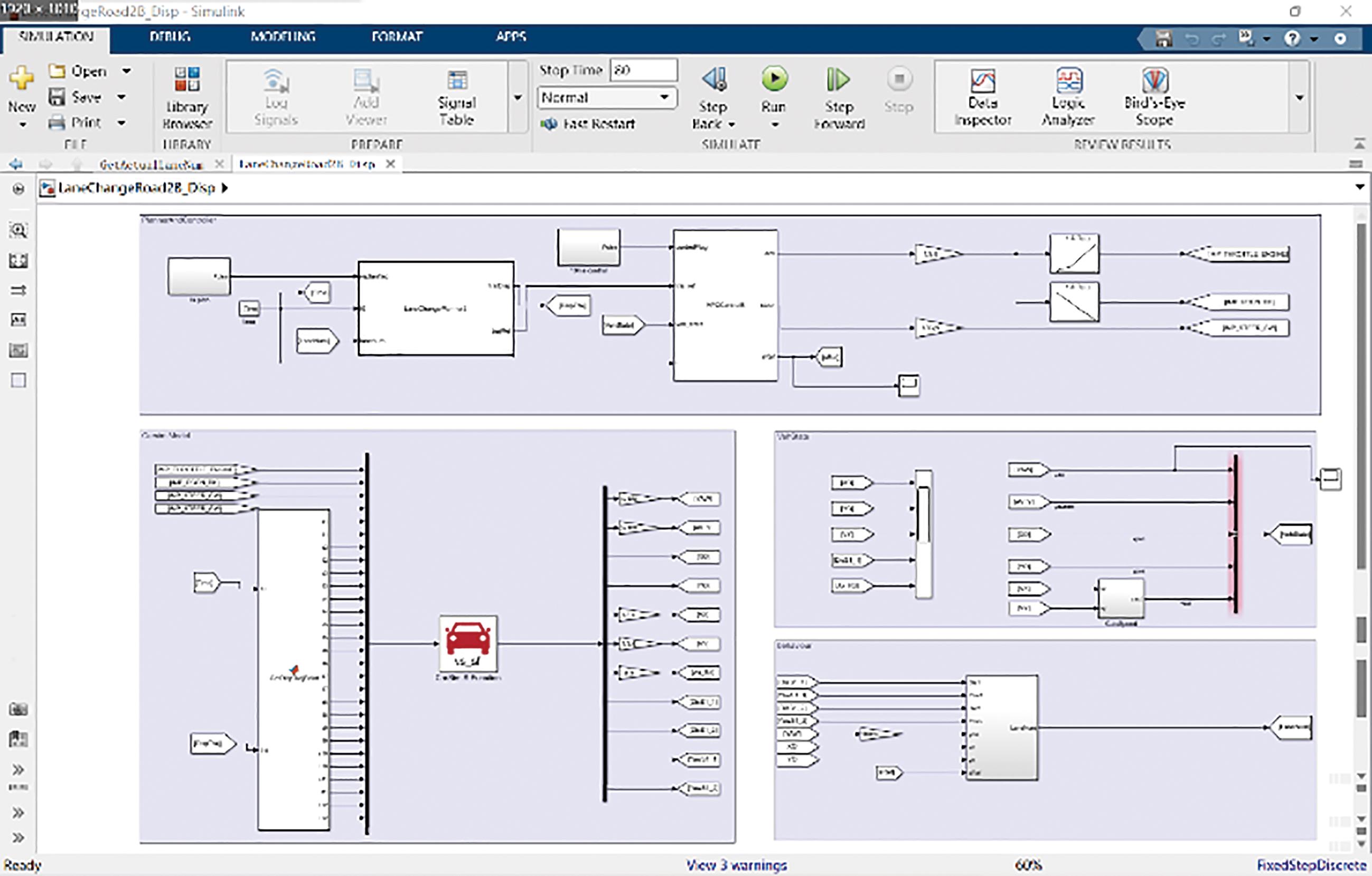
Figure 2. Co-simulation method of CarSim and Simulink.
In order to realize the tracking control of the vehicle’s high-speed lane changing trajectory, it is necessary to verify the tracking stability of the built model predictive controller in high-speed scenarios. At present, the testing of vehicle tracking characteristics mainly includes double line shifting test and serpentine penetration test. In this paper, the serpentine penetration test condition at a high speed is selected, the corresponding test scene is established in CarSim, and the reference driving trajectory is given by the control system. The test requirements for the serpentine penetration test in GB/T6323.1-94 are as follows:
For the test of small and medium-sized vehicles, the distance between the two stakes is 30 m, and the vehicle is required to pass at least 5 stake areas at a reference speed of 65 km/h.
Given the reference travel trajectory of the serpentine pole, the vehicle pass through the stake at a speed of 65 km/h is realized as required by the test, see Figure 3.
Figure 4 shows the yaw error. It can be seen that the maximum yaw angle error does not exceed 8% in the process of vehicle tracking.
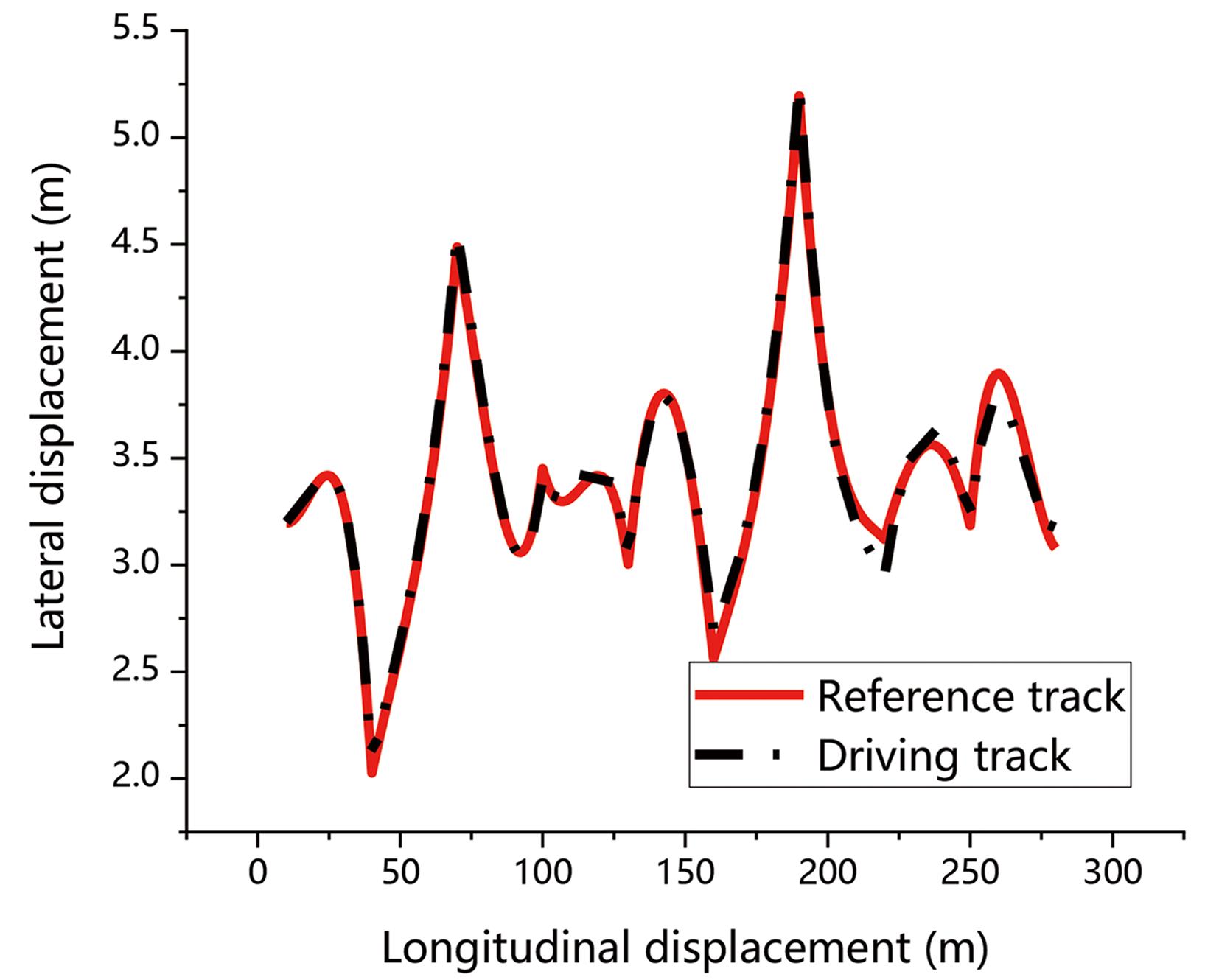
Figure 3. Simulation results of serpentine penetration road.
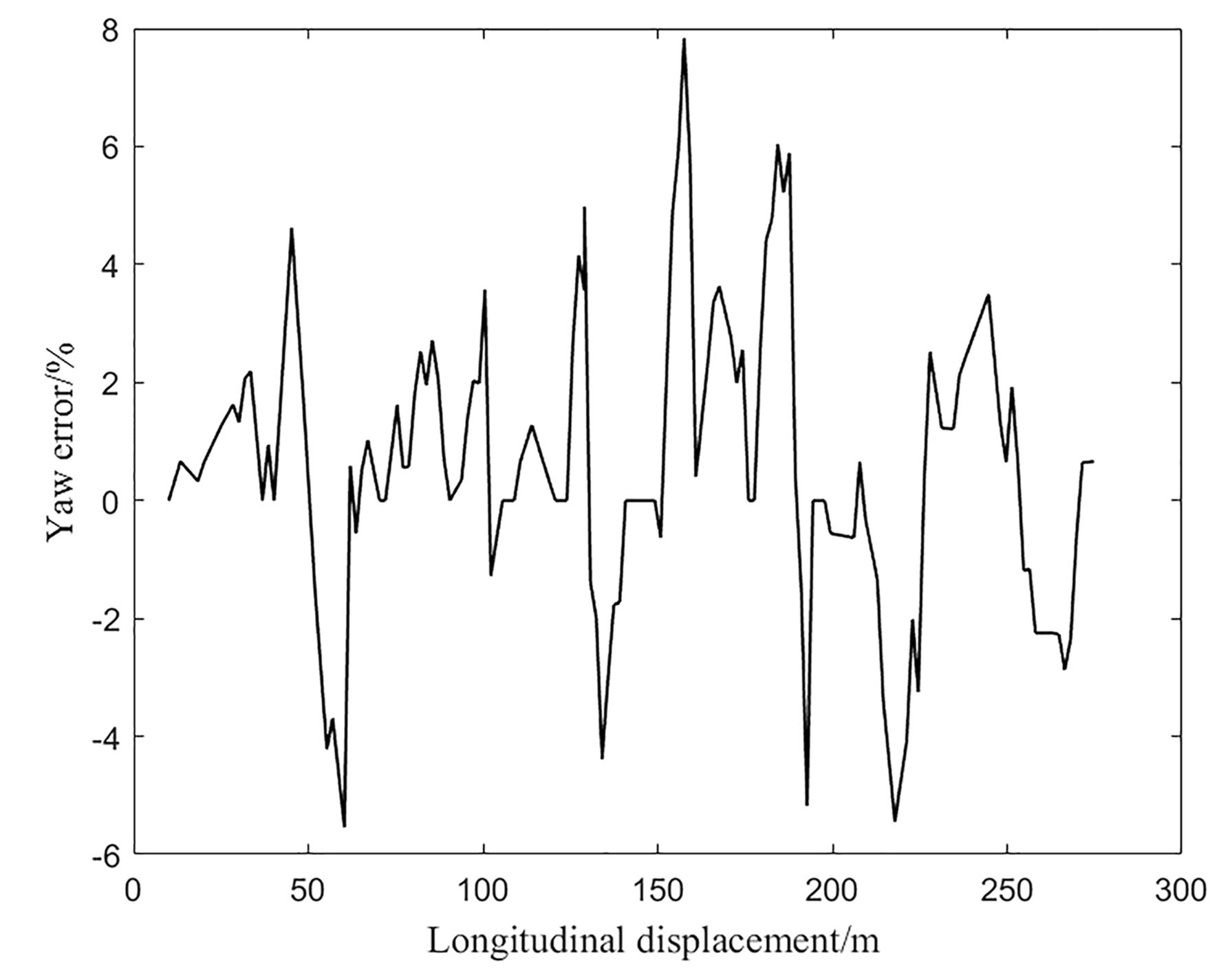
Figure 4. Simulation results of yaw error.
In the process of bypassing multiple stakes, the established model predictive controller can control the vehicle to stably track the given reference trajectory, and the tracking error is controlled in a very small range. Consequently, the model predictive controller meets the vehicle’s high-speed steering driving.
3.2.Motion Planning Simulation Analysis
From the perspective of planning, the rationality of the lane-changing trajectory is guaranteed. The planned optimal lane change trajectory will be used as the reference input for steering control, and the MPC method will be used to complete the automatic steering operation. In this section, the traffic scene of the lane-changing process will be built in CarSim, and the lane-changing process in the two scenarios of both straight and curved roads will be simulated and analyzed, so as to verify the effectiveness of the control algorithm.
The longitudinal speed curve is imported after being calculated by Matlab, and the speed control is completed by the longitudinal controller of CarSim; while the reference path of the steering is given by the S function, and the steering control is realized by the model prediction controller.
After considering the lane-changing safety distance, the planned trajectory can ensure that the lane-changing vehicle does not collide with other traffic vehicles during the entire lane-changing process. Therefore, the lane-changing model established in this paper can meet the requirements of intelligent connected vehicles to safely and stably complete the lane-changing driving task at a high speed.
When using the polynomial method to plan the lane-changing trajectory, it can satisfy the planning of the longitudinal speed and the travel path of the lane-changing at the same time. The speed curve is imported into CarSim, and the speed control curve shown in the figure below can be obtained by reasonably adjusting the relevant parameters of the vehicle speed controller. The speed control curve is shown in Figure 5.
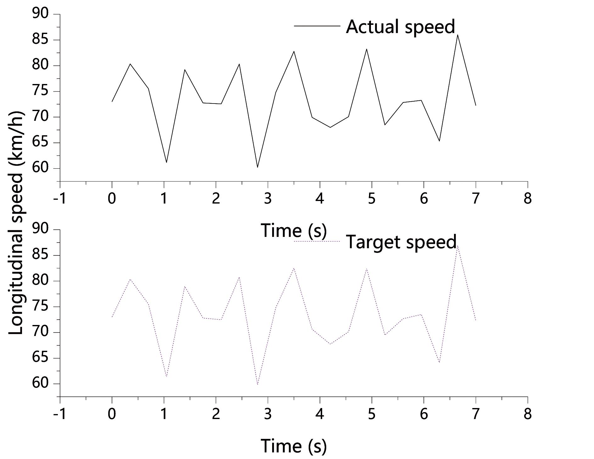
Figure 5. Speed control curve.
The planned target speed curve is relatively smooth in the whole process, which can meet the comfort requirements of the vehicle during longitudinal acceleration. The actual speed of the vehicle is basically consistent with the target speed to ensure the accuracy of speed control, so that the vehicle can meet the requirements of the spatiotemporal sequence in trajectory planning, that is, the vehicle can reach a given position at a given time.
In the model predictive controller, given its reference polynomial lane-changing trajectory, the controller parameter is set for prediction in the time domain, and the lane-changing motion planning results alongside tracking errors can be obtained as shown in Figure 6 and Figure 7, respectively.

Figure 6. Motion planning results for lane changing.
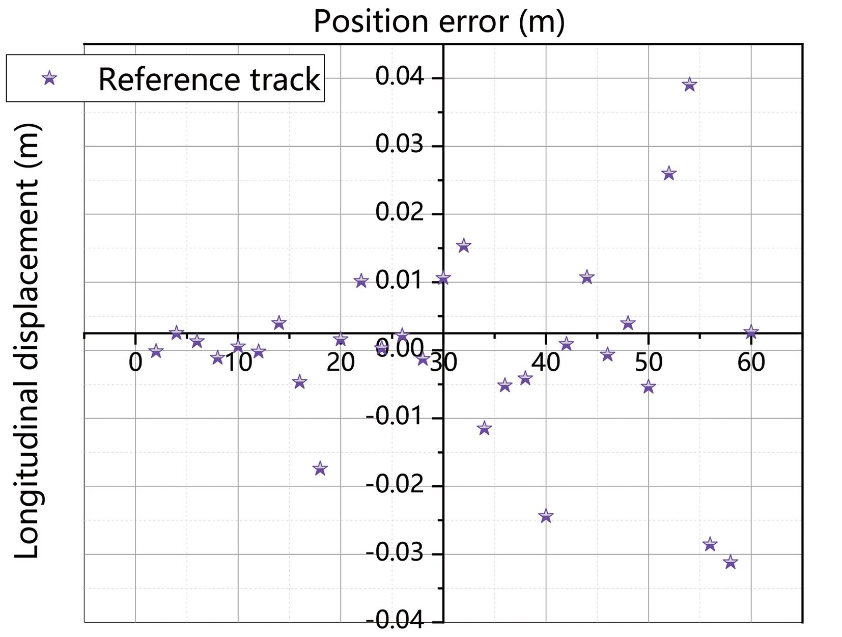
Figure 7. Motion planning error.
The model predictive controller has a good control effect in lane-changing motion planning. The lateral position error (between the trajectory of the vehicle and the reference optimal trajectory) is kept within the range of ± 0.05 m, where the control accuracy can meet the high-speed lane change of the vehicle.
It is further shown that the lane-changing trajectory using polynomial planning has better tracking characteristics, thus ensuring the coordination and unity of the planning layer and the control layer.
As for changing lanes on a curved road, since the driving conditions are more severe than those in a straight line, the vehicle is required to not turn sharply during the lane changing process, otherwise dangerous conditions such as vehicle sideslip will occur. In this case, the lane changing operation process is allowed to be completed within 6 s. Additionally, the vehicle changes its lanes at a speed of 25 m/s from a circular arc with a radius of 450 m to the left lane. The coefficients are brought into the trajectory optimization model, and the optimal lane-changing time is obtained through the golden section iteration, as shown in Figure 8.
In order to facilitate CarSim simulation, the trajectory starting point is transformed to the coordinate origin through coordinate transformation, and the trajectory points are shown in Figure 9.
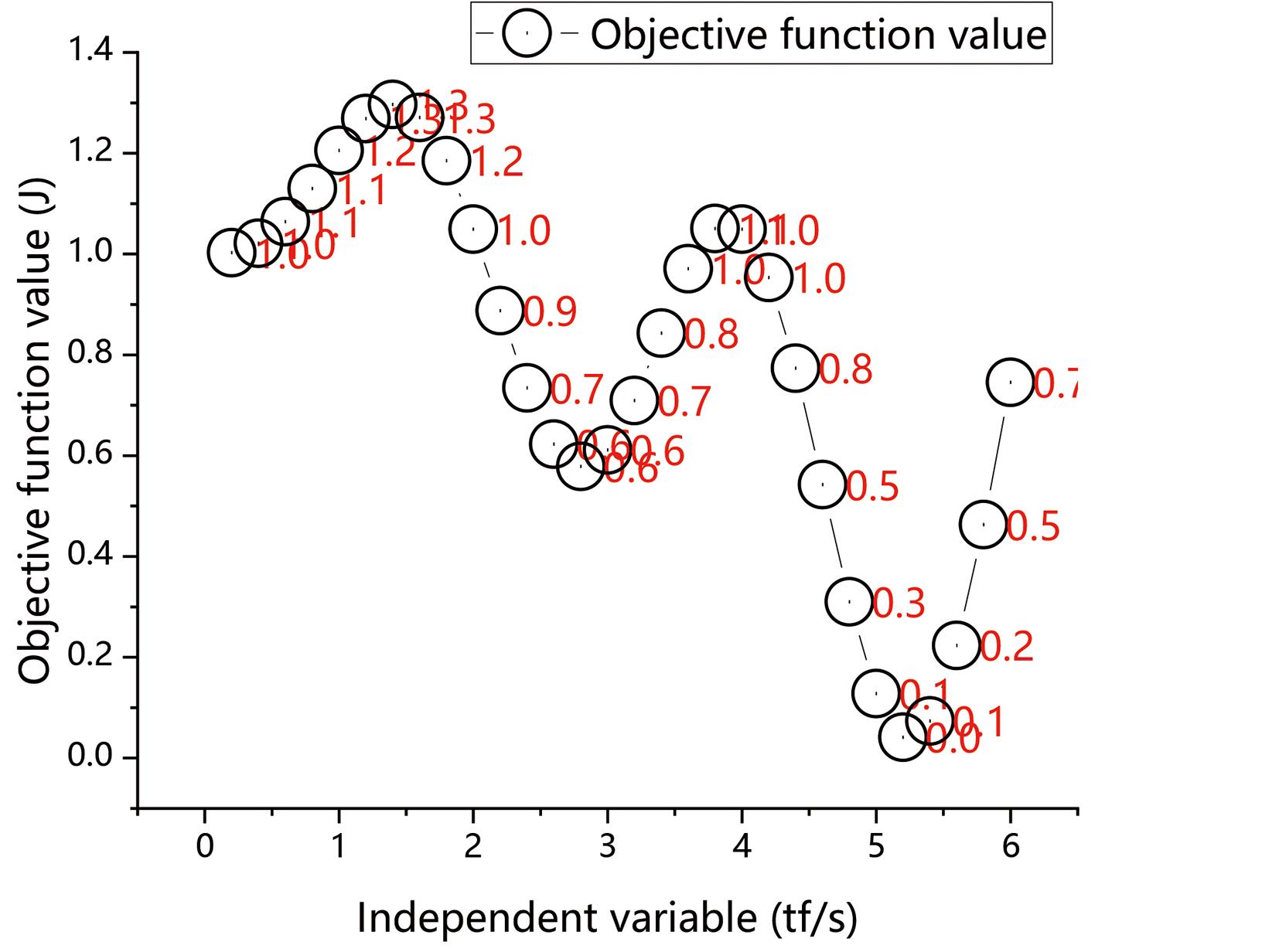
Figure 8. Objective function and its optimal solution under detours.

Figure 9. Curve point of changing lanes.
The CarSim speed controller module generates the longitudinal speed curve of the vehicle during the lane changing process, and adjusts the parameters of the speed controller reasonably. The planned target speed curve is smooth and stable, which avoids rapid changes in speed during lane changing and ensure driving comfort. The actual vehicle speed only fluctuates in a small range at the beginning, and then gradually tends to be consistent with the target vehicle speed. Overall, the speed control effect is good, which can meet the speed control requirements of the lane changing process.
4.Conclusion
This paper proposes a two-degree-of-freedom model based on the tire model to study the automatic lane changing of intelligent connected vehicles in different straight and curve situations. The proposed model provides a theoretical basis for the simulation control of vehicle lane changing and obstacle avoidance. At the same time, the trajectory tracking control is realized by the joint simulation of CarSim and Simulink, and the given reference trajectory can be tracked with high accuracy in the serpentine rod penetration test, which verifies the stability of the control algorithm.
Author Contributions: Methodology, investigation, H. W.; Writing—original draft preparation, H. W.; Software, Simulation, X. Y.; Data curation, X. Y.; Data analysis X. Y.; Writing—review and editing, Z.L.; Validation Z.W. All authors have read and agreed to the published version of the manuscript.
Funding: This work was supported by the Training Plan for Young Backbone Teachers in Colleges and Universities of Henan Province under Grant 2021GGJS032.
Data Availability Statement: The data used to support the findings of this study are available from the corresponding author upon request.
Conflicts of Interest: The authors declare that they have no known competing financial interests or personal relationships that could have appeared to influence the work reported in this paper.
References
- Zyner A. ; Worrall S. ; Nebot E . A recurrent neural network solution for predicting driver intention at unsignalized intersections. IEEE Robotics and Automation Letters, 2018, 3(3): 1759-1764. DOI: https://doi.org/10.1109/LRA.2018.2805314
- Jing S.C. ; Hui F. ; Zhao X.M. ; et al . Cooperative game approach to optimal merging sequence and on-ramp merging control of connected and automated vehicles. IEEE Transactions on Intelligent Transportation Systems, 2019, 20(11): 4234-4244. DOI: https://doi.org/10.1109/TITS.2019.2925871
- Ito Y. ; Kamal M .A.S.; Yoshimura T.; et al. Coordination of connected vehicles on merging roads using pseudo-perturbation-based broadcast control. IEEE Transactions on Intelligent Transportation Systems, 2019, 20(9): 3496-3512. DOI: https://doi.org/10.1109/TITS.2018.2876905
- van Nunen E. ; Reinders J. ; Semsar-Kazerooni E. ; et al . String stable model predictive cooperative adaptive cruise control for heterogeneous platoons. IEEE Transactions on Intelligent Vehicles, 2019, 4(2): 186-196. DOI: https://doi.org/10.1109/TIV.2019.2904418
- Noh S . Decision-making framework for autonomous driving at road intersections: safeguarding against collision, overly conservative behavior, and violation vehicles. IEEE Transactions on Industrial Electronics, 2019, 66(4): 3275-3286. DOI: https://doi.org/10.1109/TIE.2018.2840530
- Bichiou Y. ; Rakha H .A. Developing an optimal intersection control system for automated connected vehicles. IEEE Transactions on Intelligent Transportation Systems, 2019, 20(5): 1908-1916. DOI: https://doi.org/10.1109/TITS.2018.2850335
- Nilsson J. ; Brännström M. ; Fredriksson J. ; et al . Longitudinal and lateral control for automated yielding maneuvers. IEEE Transactions on Intelligent Transportation Systems, 2016, 17(5): 1404-1414. DOI: https://doi.org/10.1109/TITS.2015.2504718
- Ding J .S.Y.; Li L.; Peng H.; et al. A rule-based cooperative merging strategy for connected and automated vehicles. IEEE Transactions on Intelligent Transportation Systems, 2020, 21(8): 3436-3446. DOI: https://doi.org/10.1109/TITS.2019.2928969
- Debada G.G. ; Gillet D . Virtual vehicle-based cooperative maneuver planning for connected automated vehicles at single-lane roundabouts. IEEE Intelligent Transportation Systems Magazine, 2018, 10(4): 35-46. DOI: https://doi.org/10.1109/MITS.2018.2867529
- Hubmann C. ; Schulz J. ; Becker M. ; et al . Automated driving in uncertain environments: planning with interaction and uncertain maneuver prediction. IEEE Transactions on Intelligent Vehicles, 2018, 3(1): 5-17. DOI: https://doi.org/10.1109/TIV.2017.2788208
- Amezquita-Semprun K. ; Pradeep Y.C. ; Chen P .C.Y.; et al. Experimental evaluation of the stimuli-induced equilibrium point concept for automatic ramp merging systems. IEEE Transactions on Intelligent Transportation Systems, 2020, 21(2): 815-827. DOI: https://doi.org/10.1109/TITS.2019.2901757
- Xu H.L. ; Feng S. ; Zhang Y. ; et al . A grouping-based cooperative driving strategy for CAVs merging problems. IEEE Transactions on Vehicular Technology, 2019, 68(6): 6125-6136. DOI: https://doi.org/10.1109/TVT.2019.2910987
- de Campos G.R. ; Rossa F.D. ; Colombo A . Safety verification methods for human-driven vehicles at traffic intersections: optimal driver-adaptive supervisory control. IEEE Transactions on Human-Machine Systems, 2018, 48(1): 72-84. DOI: https://doi.org/10.1109/THMS.2017.2776205
- Pei H.X. ; Feng S. ; Zhang Y. ; et al . A cooperative driving strategy for merging at on-ramps based on dynamic programming. IEEE Transactions on Vehicular Technology, 2019, 68(12): 11646-11656. DOI: https://doi.org/10.1109/TVT.2019.2947192
- Mercy T. ; van Parys R. ; Pipeleers G . Spline-based motion planning for autonomous guided vehicles in a dynamic environment. IEEE Transactions on Control Systems Technology, 2018, 26(6): 2182-2189. DOI: https://doi.org/10.1109/TCST.2017.2739706
- Xu T. ; Wen C.L. ; Zhao L. ; et al . The hybrid model for lane-changing detection at freeway off-ramps using naturalistic driving trajectories. IEEE Access, 2019, 7: 103716-103726. DOI: https://doi.org/10.1109/ACCESS.2019.2932013