Downloads

Wang, J., Zhuang, Y., & Liu, Y. FSS-Net: A Fast Search Structure for 3D Point Clouds in Deep Learning. International Journal of Network Dynamics and Intelligence. 2023, 2(2), 100005. doi: https://doi.org/10.53941/ijndi.2023.100005

Article

FSS-Net: A Fast Search Structure for 3D Point Clouds in Deep Learning

Jiawei Wang 1, Yan Zhuang 1,*, and Yisha Liu 2,*

1 School of Control Science and Engineering, Dalian University of Technology, Dalian 116024, China

2 Information Science and Technology College, Dalian Maritime University, Dalian 116026, China

* Correspondence: zhuang@dlut.edu.cn; liuyisha@dlmu.edu.cn


Received: 22 February 2023

Accepted: 5 May 2023

Published: 23 June 2023


Abstract: 
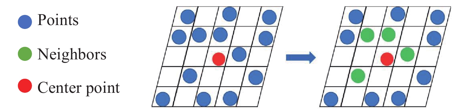
The deep learning methods achieve good results in the semantic segmentation and classification of the 3D point clouds. The popular convolutional neural networks illustrate the importance of using the neighboring information of the points. Searching the neighboring points is an important process that can get the context information of each point. The K-nearest neighbor (KNN) search and ball query methods are usually used to find the neighboring points, but a long time is required to construct the KD-tree and calculate the Euclidean distance. In this work, we introduce a fast approach (called the voxel search) to finding the neighbors, where the key is to use the voxel coordinates to search the neighbors directly. However, it is difficult to apply this method directly to the general network structure such as the U-net. In order to improve its applicability, the corresponding up-sampling and down-sampling methods are proposed. Additionally, we propose a fast search structure network (FSS-net) which consists of the feature extraction layer and the sampling layer. In order to demonstrate the effectiveness of the FSS-net, we conduct experiments on a single object in both indoor and outdoor environments. The speed of the voxel search approach is compared with that of the KNN and ball query. The experimental results show that our method is faster and can be directly applied to any point-based deep learning networks.

Keywords:

3D point cloud semantic segmentation fast search local feature extraction

1. Introduction

Semantic segmentation of the environment has been one of the most fundamental tasks in autonomous robotic systems, e.g. the mobile robots that sweep the floor, the humanoid robots that serve food in the restaurant, or the quadcopters that map and inspect an industrial factory. 3D deep learning networks have received increasing attention in these fields. In this paper, we aim to propose an approach to accelerating the network.

As for the 3D point clouds collected by the light detection and ranging (LiDAR), they are typically unordered, unstructured, and irregularly sampled. The PointNet [1] is the pioneering work that used the per-point multi-layer perception (MLP) to extract point features, and the symmetric function to extract the global feature, where the local context modeling capability was not discussed. Several point-based methods have been proposed, see [1–14]. From the perspective of traditional convolutional neural networks (CNNs), the shape information and semantic information of points are affected by the information of the surrounding points, and it is important to exploit the local structure. The above work was further extended to the PointNet++ [9]. For images, CNNs can easily obtain the neighboring points through the pixel coordinates, while for the point clouds, the neighboring points are unordered, unsampled, and unstructured. Therefore, it is impossible to directly apply CNNs to get local information (Figure 1).

Figure 1. Fast search. We voxelize all points (blue) and search neighbors (green) of a center point (red). In our method, we can quickly find neighboring points.

The PointNet++ [9] uses the farthest point sampling (FPS) [15] method to sample points of the entire point clouds. The principle of the FPS is to pick the points that maximize the distance to the selected points. Then, a radius-based ball query method is used to find the neighboring points, and a hierarchical feature learning framework is used to extract the features.

Note that calculating the Euclidean distance between points and sorting them according to the distance have the computation cost of . Ref. [8,12,16] used the method of establishing a KD-tree to search for neighboring points, which is more efficient than the method of calculating the Euclidean distance. The method of using the KD-tree has the computation cost of . In order to reduce the time cost, the author in [12] compared the FPS method with the inverse density importance sampling (IDIS) method, and proposed a random sampling method. In the process of extracting local features, the KD-tree of all points is used to obtain a fixed number of neighboring points around each down-sampling point. Inspired by image-based convolution, ref. [8] used a set of kernel points to define the area where each kernel weight was applied. When extracting the local features, it is necessary to query the neighboring points within a fixed range of the point. To search the neighbor, the KD-tree is also established for the overall point clouds.

In this paper, we propose an effective method of searching the neighboring points, where there is no need to construct the data structure, like the KD-tree. The key of our method is to create several index arrays to achieve efficient search. However, it is not applicable to a large-scale environment. We analyze the reasons and propose an improved method. In our method, we define the basic unit space and the sample space. For the basic unit space, we establish the mapping relationship between points and grids, and then process the quick search with the help of the coordinate information. A sample space is composed of 27 basic unit grids. To maintain the 3D geometric information as much as possible, we adopt a uniform sampling method, which makes the number of input points to be variable. Then, we design a complement strategy. Finally, we design the up-sampling strategy to adapt to the encoder-decoder network structure. For the overall pipeline, we follow the network structure of the RandLA-net [12] and use the feature extraction modules. In Section 3, the methods are introduced in detail.

To prove the efficiency of our proposed search method, we directly compare it with the ball query and KNN. It can be seen that our search method has less time and memory costs. To prove the universality and ability of the FSS-net, we conduct tests on three kinds of datasets: the single object, indoor environment, and outdoor environment. The details of the experiment are introduced in Section 4.

Our main contributions are summarized as follows:

• We propose a fast method of searching neighboring points. In order to improve the universality of the voxel search (VS), we design a new structure that can be embedded in any point-based method.

• We provide extensive experiments on the task of semantic segmentation and classification to prove the ability of the FSS-net.

2. Related Work

2.1. Voxel-based Method

The early voxel-based method [17,18] converted the input points into voxels and applied vanilla 3D convolution. The OctNet [19] proposed a 3D deep convolutional network of high resolution, exploited the sparsity of the point clouds, and built a new data structure. By using a set of unbalanced octrees where each leaf node stores a pooled feature representation, the OctNet partitions the point clouds hierarchically and achieves the deeper networks without compromising resolution. In order to adapt to input scenes of various scales, the work in [20] transformed the scene into certain organized internal representation that can be processed via convolution. The VoxelNet [21] is a 3D detection framework that learns to predict accurate 3D bounding boxes, where a voxel feature encoding (VFE) layer was proposed to learn complex features for local 3D shape information. This work benefits both from the sparse point structure and efficient parallel processing of the voxel grid. Instead of using the spherical of bird’s-eye-view projection, the PolarNet [22] proposed the polar representation which can balance the points in a polar coordinate system. The PolarNet also designs a special CNN to convolve continuously on the polar grid. The work in [23] predicted the significance of each local point feature based on the point context, and focused on the task-relevant feature when aggregating local features. In detail, the local features were taken and an attention map was proposed that estimates a weight for each point based on the contextual information. Based on the Minkowski engine [24], 2-S3Net [25] presented a novel multibranch attentive feature selection module where the feature map was re-weighted in the decoder. The VoxSegNet [26] proposed a network that could extract discriminative features of encoding details from 3D voxel data under limited resolution, and designed a spatial dense extraction (SDE) module and an attention feature aggregation (AFA) module for volumetric object semantic segmentation. Although efficient in data structuring, the voxel-based methods are of low accuracy when resolution is reduced.

2.2. Point-Based Method

The PointNet [1] is the first work to operate on points through the MLP network. Ref. [2–6, 9] learned to extract the local features to enhance the segmentation results. CKConv [7] proposed a spatial attention module to provide comprehensive structure awareness within the local point set, where the representative features were produced. KPConv [8] designed novel point convolution based on the spatial kernel which is more flexible than the fixed grid convolution. In [ 10], the authors proposed a semantic-instance segmentation method that jointly performs the tasks via a novel multi-task pointwise network and a multi-value conditional random field model. The RandLA-Net [12] used an efficient and lightweight neural architecture to recognize the point cloud faster. To overcome the problems caused by random sampling, the local spatial encoding (LocSE) and attentive pooling (AP) were embedded into the structure of the network to enhance the local features. For the point-based methods, the cost of data structuring becomes the performance bottleneck of large-scale point clouds.

2.3. Fusion Method

Ref. [27,28] paid attention to the point-voxel interaction MLP, and aggregated features among neighboring voxels and corresponding points. The RPVNet [29] proposed a range-point-voxel fusion framework, and designed an efficient interaction mechanism by utilizing hash mapping. In the outdoor environment, the density is varying. Motivated by this investigation, the work in [30] proposed a framework for the outdoor LiDAR segmentation, where cylindrical partition and asymmetrical 3D convolution networks were designed to extract the 3D topology and geometric relations. However, the above methods not only increase the memory, but also reduce efficiency.

2.4. Strategies for Searching Neighbors

Ref. [9,31–33] used FPS [15] to search the neighbors for each point. FPS picks the points that maximize the distance to the selected points. This method has the computation cost of . Ref. [8,12,34] built the KD-tree to search neighbors in the efficient data structure. This method has the computation cost of . RPS in [12] is the fastest strategy to sample points, but cannot work without the help of the KD-tree. Our method can search the neighbors with the computation cost of  and keep the distribution of points uniform.

In this paper, we propose a fast method of searching neighboring points and design a new structure that can be embedded in any point-based method.

3. Methods

The point cloud, captured by LiDAR, is a set of points with irregular structures, unordered arrangement, and sparse distributions. The input is the coordinate of each point  and the corresponding features , where  is the dimension of the point feature. The standard convolution operation on an arbitrary point  can be formulated as follows:

where  is the kernel function,  is the neighboring point of  is the feature of , ‘ ’ denotes the dot product, and  is the set of neighbor points of .

For the point cloud, the kernel function should be able to handle any points in the continuous space. Therefore, the kernel function is designed to get the relationship between points. Generally, the MLP is employed for the kernel function which takes the positions of neighbors (that center on ) as inputs.

Since the point cloud is unordered, it is difficult to find  of . As it is shown in the previous work, there are two main methods that can be used to obtain the neighbors. One method is to construct a KD-tree for the point clouds, and the other method is to directly calculate and sort the distance between points. We propose a method to speed up this process which has the computation cost of . As the method of searching for neighboring points is changed, we correspondingly propose new methods for up-sampling points and down-sampling points.

Similar to the network structure used in the existing work, our network structure includes the local feature extraction layers and sampling layers.

3.1. Feature Extraction Layer

Algorithm 1 and Figure 2 show the process of searching neighbors. We aim to find  neighboring points for each point. We set  as the length of the grid that divides the point cloud. We define the space of length  as the basic unit space. There is, at most, one point in the basic unit space. The size of the sampling space is set as , where  represents the number of down-sampling. For the sake of clarity, we set . When we sample points, we hope to find, at most, one point in each non-empty sampling space.

Figure 2. Search Neighbors (SN). On the left, the blue points are distributed around the central red point. The green points which are in the same sampling space as the red point are picked as the neighbors. On the right, we randomly pick the neighbors to supplement.

When the program is initialized,  is defined to mark whether there is a point in each grid. If there is a point in this grid, we set the corresponding position in the  as 1; otherwise, we set it as 0.  is declared to store the distribution of points in the sample space. In the following processing, we consider the unit grid in the sampling space as a local area and extract the local features of points.  is the return value, which is used to store the indexes of neighbors.

For the  point, its coordinates are , and the index in the basic unit space is  which are defined as follows:

We set the corresponding position in the  as 1 according to Equation (3). With the help of this array, we can ensure that only one point in each grid is accessed. Then, we calculate the position of the point in the sampling space, which is defined in Equation (4).

We add the index of this point to the  according to . Then, we calculate the position in the sampling space for each point again, and set points in this position as the neighbors. Note that the number of neighbors of each point is different, but fixed. We unify the neighbor numbers of all points. For each point, we regard itself as a neighboring point. Therefore, every point has at least one neighbor. For points whose number of neighbors does not meet , we assume that the number of existing neighbors is , and then randomly select  points from the existing neighboring points.

Finally, we get  which contains the neighbor indexes of each point. In the neural network, the neighboring points corresponding to each point can be obtained directly with the help of .

There is a very important part in this algorithm. We define many dynamic arrays to calculate . For the arrays with large sizes, it takes a lot of time to initialize them. Different from the general initialization methods of dynamic arrays, we only declare the starting address and the size of arrays in the program, which results in the randomness of the initial data in the arrays. However, due to the characteristics of Algorithm 1, the randomness of the data does not affect the accuracy of the algorithm. In addition, to improve the execution speed of the program, we use the g++ compiler to generate a static library which can be found in Python.

We use two basic structures from the RandLA-Net: the local spatial encoding and attentive pooling structures.

1) Local Spatial Encoding (LSE): For the  point and its  neighbors , we encode the relative point position as follows:

where  and  are the coordinates of points,  is the concatenation operation, and  calculates the Euclidean distance between the  neighbor and the center point. We add a negative exponential term of the distance from the neighbors to the center point. Compared to distant neighbors, we expect to get richer information from close neighbors.

For each neighbor , we concatenate its encoded relative point position  with its corresponding point feature  to obtain an augmented feature vector . For LSE, it outputs the neighboring point features  of the center point .

2) Attentive Pooling (AP): Given the features from , this module uses a function  that consists of a shared MLP followed by softmax, and is defined as follows:

where  is the learnable weights, and  is regarded as a soft mask which can select the important features. Then, these features are summed as follows:

At last, we use the residual block to connect these two modules and get the local features of the input points from neighboring points.

3.2. Sampling Layer

The down-sampling process corresponds to Figure 3, and the up-sampling process corresponds to Figure 4. Algorithm 2 includes both of them.

Figure 3. Uniform Down-sampling(UD). We only randomly pick one point as the down-sampling point in a sample space. Then we randomly expand down-sampling points to supplement.

Figure 4. Up-Sampling(US). Similar to SN, the green points are the neighbors of the red point. We randomly select a yellow point from green points as the up-sampling point.

For the process of down-sampling points, we expect to adopt an average sampling method so that the sampled points cover all areas. However, such a method will cause the number of down-sampling points to be variable. Therefore, it is necessary to adaptively increase the existing points. In the up-sampling process, for each point, we randomly select a point in the same sample space as the up-sampling point.

We set  with length  to save the indexes of the down-sampling points.  is the preset number of down-sampling points. We define  of size  to save the neighbors of the down-sampling points, and  of size  to save the indexes of the up-sampling points.

In Algorithm 2, for each point, we calculate its position in the sample space. If we visit this position for the first time, we set this point as the down-sampling point of this position and update the access status of this position. Then, we finish the uniform sampling process and put the indexes of down-sampling points into . If the size of  is smaller than , we randomly expand the indexes in  until the size is equal to ; Otherwise, the input points cannot be uniformly sampled.

In Algorithm 1, we use its coordinates to calculate the position in the sampling space to obtain the neighboring points of each point. We set all the points at this position as its neighbors. However, this method is not the best.

Similarly, we define the  point and its neighbors as . In the process of searching neighboring points, we ignore the relative position between  and , which means that  may be anywhere, e.g. the corner, edge, and center. This will reduce the ability of the kernel function to extract local features. Therefore, we change the method of finding neighboring points.

We search the neighboring grids of each point. With the help of the  in Algorithm 1, we can get the distribution of surrounding points. Then, we set the points centered at this point as the neighbors. This process is shown in Figure 5.

Figure 5. Search Neighbors (SN). On the left, the blue points are distributed around the central red point. The green points around the red point are picked as the neighbors. On the right, we randomly pick the neighbors to supplement, where N*D represent the shape of point features.

3.3. Limitations of VS

In VS, we define several search arrays based on the entire space, where arrays defined in C++ are limited in size. Each array cannot be larger than 0x7fffffff bytes. This limits the size of the point cloud space. In the SemanticKITTI dataset, points in the autonomous driving environment are sparsely distributed. We set the network input point as 40960. If the space represented by these points is too large, our algorithm will overflow. Thus, we use a hash table (instead of an array) to store each coordinate, which makes our method still effective in case of large spaces.

In a sparse environment,  in Algorithm 2 may be greater than . This indicates that the number of the sampling spaces is larger than the preset sampling points and there are some redundant sampling spaces, which leads to the failure of uniform sampling and up-sampling. Therefore, we divide the sampling space into two parts. The first part consists of the pre-sampled points of size , which is defined as . The second part consists of the redundant points of size , which is defined as . For each point in , we find the closest point in . Then, we map the up-sampling points of this sampling space in  to the point in , see Figure 6.

Figure 6. The left figure is the basic unit space, and the right figure is the sampling space. Each sample grid contains multiple basic grids. We perform uniform sampling in the base unit space. In the sampling space, the red points belong to  and the black points belong to . For each point in , we find the nearest point in , and then the upsampled points of the black point are mapped to .

For the decoding part of the neural network, we concatenate the corresponding low-level features with high-level features. The whole network structure is shown in Figure 7. The EL consists of the methods of searching neighbors and uniform down-sampling, and the modules of the LSE and AP. The DL consists of the US method and concatenates the features from the EL.

Figure 7. (a) is defined as the encoder layer (EL), (b) is defined as the decoder layer (DL), and (c) is the network structure.

For the total objective of our method, we only use the weighted cross-entropy loss to supervise the training, which can be formulated as

where  is defined as the percentage of points in a certain category to the total points,  is the predicted value by the prediction model, and  is the true value.

For the objects with a small number of points, the loss function can draw higher attention through .

4. Experiments

In the experiment, we use three datasets, i.e. the ModelNet40, S3DIS, and SemanticKITTI.

The ModelNet40 contains 9843 train models and 2468 test models. We first sample 1024 points (from the original 10000 points) as inputs and add normal information. We use voxel sampling [8,12] in the preprocessing sampling and calculate the index of points without adding any complexity. For each point, the final input contains coordinates, normal and indexes. For the indexes, they do not participate in the training process, and only play a role in the process of searching neighbors.

The S3DIS dataset [35] consists of 271 rooms that belong to 6 large areas. Each point is annotated with one semantic label from 13 classes. We follow the sampling strategy used in [12] to prepare the training data. The difference is that we add indexes information to each point which is represented by a 9D vector combining the XYZ, RGB, and indexes.

The SemanticKITTI dataset [36] consists of 21 sequences and 28 categories of objects. We train the sequences 00~07 and 09~10, and validate the sequence 08. We sample the SemanticKITTI like the S3DIS in the preprocessing and add the indexes.

We divide the experiments into two parts, where the first part proves the efficiency of the search method and the second part proves the ability of our network. Note that the method that exploits the search array is defined as method A, and the method that uses the hash table is defined as method B. All experiments are conducted on an Intel i7-10700F CPU and an NVIDIA RTX1070 GPU.

4.1. The Efficiency of Our Search Methods

We compare our search method with the ball query and KNN methods.

The time comparison results are shown in Figure 8. For the ball query method, we combine it with FPS. For the KNN search, we combine it with the random sample. In method A, we use the SN in Figure 5, the US in Figure 4, and the DS in Figure 3. Method B is similar to method A. The difference is that we use a hash table instead of a search array. The up-sampling strategy is also replaced by the method described in Figure 6. For the test dataset, we test on the ModelNet40. We take a different number of points as inputs and set the sampling ratio as 10. Since the performance of the network is not considered in this experiment, the number of sampling layers is set as 1.

Figure 8. Time comparison experiment of the VS, ball query, and KNN on ModelNet40.

It can be seen that our method is 350 times faster than the ball query method and nearly 10 times faster than the KNN method. The more input points, the more obvious the effect of our method. Method A and method B show similar performance. In addition, the KNN method outperforms the ball query method, and has the same memory consumption as our methods.

In order to test the efficiency of our search method on a large scale environment, we compare method B with the KNN on SemanticKITTI. The result is shown in Table 1. We set the number of input points to be 40960, the number of layer to be 4, and the sample ratio to be 4. It can be seen that method B is 3 times better than the KNN. Here, we analyze the ball query method, KD-tree method and our proposed method. For the ball query method, it calculates the Euclidean distances between every two points in the whole point clouds, where the distances are sorted by size and the computational complexity is . For the KD-tree, it is similar to a high dimensional binary search tree. The time complexity of building a KD-tree is . In the worst case, the time complexity of searching neighbors is . For our method, we encode the coordinates first, and then use the hash table for query neighbors. The time complexity of the query is . To sum up, our search method shows certain advantages in both theory and experiment.

Table 1. Time comparison experiment of method B and the KNN on SemanticKITTI

  VS KNN
time consumption(s) 0.065 0.17


4.2. The Ability of FSS-Net

In this section, we test the FSS-net on the ModelNet40, S3DIS, and SemanticKITTI. Due to the limited usage scenarios of method A, we only insert method B into the FSS-net.

4.2.1. ModelNet40

The experiment based on the ModelNet40 is shown in Table 2, where the overall accuracy (OA, ) and mean of class-wise accuracy (mAcc, ) are reported. We set the batch size to be 12 and the number of input points to be 5120. The point cloud is downsampled with a two-fold decimation ratio.

Table 2. Object classification results on ModelNet40

Methods OA( ) mAcc( )
SO-NET [16] 90.9 87.3
KCNet [37] 91.0 -
PointCNN [31] 92.2 88.1
PointNet [1] 89.2 86.2
PointNet++ [9] 91.9 -
CKConv [7] 93.2 90.4
PointNet++(without normal [9]) 90.7 -
Our sampling method + PointNet++ 89.5 85.9
FSS-Net 91.2 87.0
FSS-Net(without normal) 90.3 86.5

For the accuracy of the classification experience, our proposed method is not the best. We think the reason is that, the number of neighboring points obtained by the ball query or KNN is sufficient, but the searching range of our method is the closest grids. We cannot get enough neighbors when the distribution of points is sparse. Although we use the method of randomly expanding the neighboring points, it still cannot compensate for the lack of neighbors.

Theoretically, VSd can be applied to any point-based deep learning network, and thus it is applied to the PointNet++. Although the accuracy is sacrificed, the efficiency is improved according to the experiment in Figure 6.

Based on ModelNet40, the effect of changing grid sizes on the search method is analyzed in Table 4 and Figure 9. In Figure 9, we count the distribution of the number of neighbors with different grid sizes. The grid size is defined as the size of voxel sampling used in preprocessing. The abscissa indicates the number of neighboring points. The ordinate represents the percentage of points (with different numbers of neighbors) to the current point cloud. The distribution of neighboring points will change with the grid size. Classification results on different grid sizes are shown in Table 4. If the grid size is too small, then the number of neighboring points is not enough. If the grid size is too large, information loss may occur. As such, it is necessary to choose an appropriate sampling size.

Figure 9. We set the max number of neighbors as 20 and count the distribution of the number of neighbors with different grid sizes.

4.2.2. S3DIS

The results of semantic segmentation are shown in Table 3. The overall accuracy (OA, ) and mean of class-wise accuracy (mAcc, ) are reported. We set the batch size to be 3, the number of input points to be 40960, and the network layer to be 5. The point cloud is sampled at a 4-fold sampling ratio.

Table 3. Semantic segmentation results on S3DIS

Methods OA(%) mIoU(%) ceil. floor wall beam col. wind. door chair table book. sofa board clut.
Pointnet [1] - 41.1 88.8 97.3 69.8 0.1 3.9 46.3 10.8 52.6 58.9 40.3 5.9 26.4 33.2
Segcloud [38] - 48.9 90.1 96.1 69.9 0 18.4 38.4 23.1 75.9 70.4 58.4 40.9 13 41.6
Eff-conv [39] - 48.9 90.1 96.1 69.9 0 18.4 38.4 23.1 75.9 70.4 58.4 40.9 13 41.6
pointCNN [31] 85.9 57.3 92.3 98.2 79.4 0 17.6 22.8 62.1 74.4 80.6 31.7 66.7 62.1 56.7
Pointweb [40] 87 60.3 92 98.5 79.4 0 21.1 59.7 34.8 76.3 88.3 46.9 69.3 64.9 52.5
Fpconv [41] 88.3 62.8 94.6 98.5 80.9 0 19.1 60.1 48.9 80.6 88 53.2 68.4 68.2 54.9
Kpconv [8] - 67.1 92.8 97.3 82.4 0 23.9 58 69 91 81.5 75.3 75.4 66.7 58.9
Ckconv [7] 89.5 67.1 94.1 98.6 84.1 0.1 35.6 58.6 64.3 79.7 89.2 60.8 70.5 81.2 55.7
FSS-Net 84.9 55.08 90.32 97.18 76.9 0 15.24 56.99 26.9 81.65 72 65.03 30.8 57.81 45.2

Table 4. Classification results on ModelNet40 with different grid sizes

Grid size OA( ) mAcc( )
0.2*0.2*0.2 89.0 85.0
0.3*0.3*0.3 91.2 87.0
0.4*0.4*0.4 90.5 86.8

Based on S3DIS, we compare the methods of searching neighbors proposed in Figure 2 with the improved method proposed in Figure 5, and the comparative results are shown in Table 5. The overall accuracy (OA, ) and mean of instance-wise (mIoU, ) are reported. It can be seen that the results of the improved method outperform that of the searching method when the neighboring points are evenly distributed.

Table 5. Semantic segmentation results on S3DIS with different methods of searching neighbors

Sampling method OA( ) mIoU( )
Figure 2 78.1 44.0
Figure 5 84.9 55.1


In the training process, we add weights to the loss to improve the classification results of objects with a small number of points. The result is shown in Table 8. To highlight the efficiency of the local spatial encoding module, we provide the results of the ablation study shown in Table 7. To simplify the representation, we define  as . Different from the general local spatial module, we add a negative exponential term (of the distance from the neighbors) to the center point. We expect the input value of the close points to be larger, and the value of the far points to be smaller. This exponential term can satisfy the above requirements and can also ensure that the inputs are distributed in the 0-1 interval. Meanwhile, the exponential term does not affect the speed of convergence or cause the data scale problem. It can be seen from the experimental results that the added exponential term is effective.

4.2.3. SemanticKITTI

We set the batch size to be 2, the number of input points to be 45056, and the network layer to be 4. The point cloud is sampled at a 4-fold sampling ratio. The segmentation results are shown in Table 6. In the experiment, it can be seen that our method has achieved relatively poor performance, where the performance of segmentation for each category is poor. For the data of KITTI, it belongs to the large-scaled outdoor sparse point clouds. In the process of obtaining local features, the coverage of searching neighbors is too small to extract rich local features. It is an important factor that our approach is not suitable for such sparse point clouds. In future work, we will consider more efficient local feature extraction methods.

Table 6. Semantic segmentation results on SemanticKITTI

Table 7. Ablation study

OA( ) mIoU(%)
      81.2 51.0
    82.5 52.3
  84.3 54.0
84.9 55.1

Table 8. Effectiveness of weight loss

  OA( ) mIoU( )
without weight loss 82.3 50.5
add weight loss 84.9 55.1

5. Limitations

In the domain of point-based semantic segmentation networks, we propose a novel approach to searching neighboring points, which can achieve better searching performance than the KNN approach. However, as shown in the above experiment, it is difficult to achieve better segmentation performance. The main reason is that the searching coverage is too small which only covers the adjacent voxel grids, while for the KNN, its searching range is the entire point cloud space, where richer local features can be extracted. Moreover, the number of input points at our local feature extraction module is fixed. In our network, under the condition of insufficient neighboring points, we simply copy the neighbors that have been found. The local feature extraction method mentioned in our paper may not be the most efficient for such inputs. In the future work, we will look for more efficient feature extraction methods.

6. Conclusion

In this paper, the FSS-net has been proposed which includes a fast search method for 3D point clouds and the corresponding up-sampling and down-sampling method. These methods take less time and less memory. Moreover, they can be added to other point-based deep learning networks. We have added a new exponential term to the general local space encoding module to improve the accuracy. In the experiment, we have used three datasets to conduct experiments on search efficiency, classification, and semantic segmentation. From the experimental results, we have seen that our network architecture does not achieve the most advanced performance.

Our feature extraction mainly uses the attention mechanism. In the future, we want to introduce more powerful feature extraction modules, such as the transformer, to enhance network performance. In particular, the transformer model, which uses self-attention layers, has shown remarkable performance in NLP tasks. By introducing the transformer architecture into our feature extraction module, we believe that we can further improve the network's ability to capture complex patterns and relationships in the data. In addition to improving the feature extraction module, we also plan to design a more effective loss function for the network. The loss function plays a crucial role in guiding the network's learning process and improving its performance. By designing a more effective loss function that is tailored to the specific task and data, we can further enhance the network's learning and generalization ability.

Overall, we believe that by incorporating more powerful feature extraction modules and designing better loss functions, we can continue to push the boundaries of our network and achieve even better performance in a wide range of tasks.

Author Contributions:  Jiawei Wang: investigation,  resources,  writing –original  draft  and  writing –review  & editing; Yan Zhuang: supervision; Yisha Liu: supervision. All authorshave read and agreed to the published version of the manuscript.

Funding:  This  work  was  supported  in  part  by  the  National  Key  Research  and  Development  Program  of  China

(Grant No. 2020YFC1511704) and the National Natural Science Foundation of China under Grant 61973049.

Data Availability Statement:  Not applicable.

Conflicts of Interest:  The authors declare no conflict of interest.

References

  1. Qi, R.Q.; Su, H.; Kaichun, M.; et al. PointNet: Deep learning on point sets for 3D classification and segmentation. In Proceedings of 2017 IEEE Conference on Computer Vision and Pattern Recognition, Honolulu, HI, USA, 21–26 July 2017; IEEE: New York, 2017; pp. 77–85. doi: 10.1109/CVPR.2017.16
  2. Zhang, J.Z.; Zhu, C.Y.; Zheng, L.T.; et al. Fusion-aware point convolution for online semantic 3D scene segmentation. In Proceedings of 2020 IEEE/CVF Conference on Computer Vision and Pattern Recognition, Seattle, WA, USA, 13–19 June 2020; IEEE: New York, 2020; pp. 4533–4542. doi: 10.1109/CVPR42600.2020.00459
  3. Zhang, C.J.; Xu, S.H.; Jiang, T.; et al. Integrating normal vector features into an atrous convolution residual network for LiDAR point cloud classification. Remote Sen., 2021, 13: 3427.
  4. Wang, Y.; Sun, Y.B.; Liu, Z.W.; et al. Dynamic graph CNN for learning on point clouds. ACM Trans. Graphics, 2019, 38: 146.
  5. Yan, X.; Zheng, C.D.; Li, Z.; et al. PointASNL: Robust point clouds processing using nonlocal neural networks with adaptive sampling. In Proceedings of 2020 IEEE/CVF Conference on Computer Vision and Pattern Recognition, Seattle, WA, USA, 13–19 June 2020; IEEE: New York, 2020; pp. 5588–5597. doi: 10.1109/CVPR42600.2020.00563
  6. Wu, W.X.; Qi, Z.A.; Li, F.X. PointConv: Deep convolutional networks on 3D point clouds. In Proceedings of 2019 IEEE/CVF Conference on Computer Vision and Pattern Recognition, Long Beach, CA, USA, 15–20 June 2019; IEEE: New York, 2019; pp. 9613–9622. doi: 10.1109/CVPR.2019.00985
  7. Woo, S.; Lee, D.; Lee, J.; et al. CKConv: Learning feature voxelization for point cloud analysis. arXiv: 2107.12655, 2021. doi: 10.48550/arXiv.2107.12655
  8. Thomas, H.; Qi, C.R.; Deschaud, J.E.; et al. KPConv: Flexible and deformable convolution for point clouds. In Proceedings of 2019 IEEE/CVF International Conference on Computer Vision, Seoul, Korea (South), 27 October 2019 - 02 November 2019; IEEE: New York, 2019; pp. 6410–6419. doi: 10.1109/ICCV.2019.00651
  9. Qi, C.R.; Yi, L.; Su, H.; et al. PointNet++: Deep hierarchical feature learning on point sets in a metric space. In Proceedings of the 31st International Conference on Neural Information Processing Systems, Long Beach, California, USA, 4–9 December 2017; Curran Associates Inc: Red Hook, 2017; pp. 5105–5114.
  10. Pham, Q.H.; Nguyen, T.; Hua, B.S.; et al. JSIS3D: Joint semantic-instance segmentation of 3D point clouds with multi-task pointwise networks and multi-value conditional random fields. In Proceedings of 2019 IEEE/CVF Conference on Computer Vision and Pattern Recognition, Long Beach, CA, USA, 15–20 June 2019; IEEE: New York, 2019; pp. 8819–8828. doi: 10.1109/CVPR.2019.00903
  11. Lei, H.; Akhtar, N.; Mian, A. Octree guided CNN with spherical kernels for 3D point clouds. In Proceedings of 2019 IEEE/CVF Conference on Computer Vision and Pattern Recognition, Long Beach, CA, USA, 15–20 June 2019; IEEE: New York, 2019; pp. 9623–9632. doi: 10.1109/CVPR.2019.00986
  12. Hu, Q.Y.; Yang, B.; Xie, L.H.; et al. RandLA-Net: Efficient semantic segmentation of large-scale point clouds. In Proceedings of 2020 IEEE/CVF Conference on Computer Vision and Pattern Recognition, Seattle, WA, USA, 13–19 June 2020; IEEE: New York, 2020; pp. 11105–11114. doi: 10.1109/CVPR42600.2020.01112
  13. Engelmann, F.; Bokeloh, M.; Fathi, A.; et al. 3D-MPA: Multi-proposal aggregation for 3D semantic instance segmentation. In Proceedings of 2020 IEEE/CVF Conference on Computer Vision and Pattern Recognition, Seattle, WA, USA, 13–19 June 2020; IEEE: New York, 2020; pp. 9028–9037. doi: 10.1109/CVPR42600.2020.00905
  14. Atzmon, M.; Maron, H.; Lipman, Y. Point convolutional neural networks by extension operators. ACM Trans. Graphics, 2018, 37: 71.
  15. Eldar, Y.; Lindenbaum, M.; Porat, M.; et al. The farthest point strategy for progressive image sampling. IEEE Trans. Image Process., 1997, 6: 1305−1315.
  16. Li, J.; Chen, B.M.; Lee, G.H. SO-Net: Self-organizing network for point cloud analysis. In Proceedings of 2018 IEEE/CVF Conference on Computer Vision and Pattern Recognition, Salt Lake City, UT, USA, 18–23 June 2018; IEEE: New York, 2018; pp. 9397–9406. doi: 10.1109/CVPR.2018.00979
  17. Maturana, D.; Scherer, S. VoxNet: A 3D convolutional neural network for real-time object recognition. In Proceedings of 2015 IEEE/RSJ International Conference on Intelligent Robots and Systems (IROS), Hamburg, Germany, 28 September 2015–02 October 2015; IEEE: New York, 2015; pp. 922–928. doi: 10.1109/IROS.2015.7353481
  18. Qi, C.R.; Su, H.; Nießner, M.; et al. Volumetric and multi-view CNNs for object classification on 3D data. In Proceedings of 2016 IEEE Conference on Computer Vision and Pattern Recognition, Las Vegas, NV, USA, 27–30 June 2016; IEEE: New York, 2016; pp. 5648–5656. doi: 10.1109/CVPR.2016.609
  19. Riegler, G.; Osman Ulusoy, A.; Geiger, A. OctNet: Learning deep 3D representations at high resolutions. In Proceedings of 2017 IEEE Conference on Computer Vision and Pattern Recognition, Honolulu, HI, USA, 21–26 July 2017; IEEE: New York, 2017; pp. 6620–6629. doi: 10.1109/CVPR.2017.701
  20. Rethage, D.; Wald, J.; Sturm, J.; et al. Fully-convolutional point networks for large-scale point clouds. In Proceedings of the 15th European Conference on Computer Vision (ECCV), Munich, Germany, 8–14 September 2018; Springer: Cham, 2018; pp. 625–640. doi: 10.1007/978-3-030-01225-0_37
  21. Zhou, Y.; Tuzel, O. VoxelNet: End-to-end learning for point cloud based 3D object detection. In Proceedings of 2018 IEEE/CVF Conference on Computer Vision and Pattern Recognition, Salt Lake City, UT, USA, 18–23 June 2018; IEEE: New York, 2018; pp. 4490–4499. doi: 10.1109/CVPR.2018.00472
  22. Zhang, Y.; Zhou, Z.X.; David, P.; et al. PolarNet: An improved grid representation for online LiDAR point clouds semantic segmentation. In Proceedings of 2020 IEEE/CVF Conference on Computer Vision and Pattern Recognition, Seattle, WA, USA, 13–19 June 2020; IEEE: New York, 2020; pp. 9598–9607. doi: 10.1109/CVPR42600.2020.00962
  23. Zhang, W.; Xiao, C.X. PCAN: 3D attention map learning using contextual information for point cloud based retrieval. In Proceedings of 2019 IEEE/CVF Conference on Computer Vision and Pattern Recognition, Long Beach, CA, USA, 15–20 June 2019; IEEE: New York, 2019; pp. 12428–12437. doi: 10.1109/CVPR.2019.01272
  24. Choy, C.; Gwak, J.Y.; Savarese, S. 4D spatio-temporal ConvNets: Minkowski convolutional neural networks. In Proceedings of 2019 IEEE/CVF Conference on Computer Vision and Pattern Recognition, Long Beach, CA, USA, 15–20 June 2019; IEEE: New York, 2019; pp. 3070–3079. doi: 10.1109/CVPR.2019.00319
  25. Cheng, R.; Razani, R.; Taghavi, E.; et al. (AF)2-S3Net: Attentive feature fusion with adaptive feature selection for sparse semantic segmentation network. In Proceedings of 2021 IEEE/CVF Conference on Computer Vision and Pattern Recognition, Nashville, TN, USA, 20–25 June 2021; IEEE: New York, 2021; pp. 12542–12551. doi: 10.1109/CVPR46437.2021.01236
  26. Wang, Z.; Lu, F. VoxSegNet: Volumetric CNNs for semantic part segmentation of 3D shapes. IEEE Trans. Vis. Comput. Graph., 2020, 26: 2919−2930.
  27. Liu, Z.J.; Tang, H.T.; Lin, Y.J.; et al. Point-voxel CNN for efficient 3D deep learning. In Proceedings of the 33rd International Conference on Neural Information Processing Systems, Vancouver, BC, Canada, 8–14 December 2019; Curran Associates Inc: Red Hook, 2019; p. 87.
  28. Tang, H.T.; Liu, Z.J.; Zhao, S.Y.; et al. Searching efficient 3D architectures with sparse point-voxel convolution. In Proceedings of 16th European Conference on Computer Vision, Glasgow, UK, 23–28 August 2020; Springer: Cham, 2020; pp. 685–702. doi: 10.1007/978-3-030-58604-1_41
  29. Xu, J.Y.; Zhang, R.X.; Dou, J.; et al. RPVNet: A deep and efficient range-point-voxel fusion network for LiDAR point cloud segmentation. In Proceedings of 2021 IEEE/CVF International Conference on Computer Vision, Montreal, QC, Canada, 10–17 October 2021; IEEE: New York, 2021; pp. 16004–16013. doi: 10.1109/ICCV48922.2021.01572
  30. Zhu, X.G.; Zhou, H.; Wang, T.; et al. Cylindrical and asymmetrical 3D convolution networks for LiDAR-based perception. IEEE Trans. Pattern Anal. Mach. Intell., 2022, 44: 6807−6822.
  31. Li, Y.Y.; Bu, R.; Sun, M.C.; et al. PointCNN: Convolution on X-transformed points. In Proceedings of the 32nd International Conference on Neural Information Processing Systems, Montréal, Canada, 3–8 December 2018; Curran Associates Inc: Red Hook, 2018; pp. 828–838.
  32. Liu, Y.C.; Fan, B.; Xiang, S.M.; et al. Relation-shape convolutional neural network for point cloud analysis. In Proceedings of 2019 IEEE/CVF Conference on Computer Vision and Pattern Recognition, Long Beach, CA, USA, 15–20 June 2019; 2019; pp. 8887–8896. doi: 10.1109/CVPR.2019.00910
  33. Wang, C.; Samari, B.; Siddiqi, K. Local spectral graph convolution for point set feature learning. In Proceedings of the 15th European Conference on Computer Vision (ECCV), Munich, Germany, 8–14 September 2018; Springer: Cham, 2018; pp. 56–71. doi: 10.1007/978-3-030-01225-0_4
  34. Klokov, R.; Lempitsky, V. Escape from cells: Deep Kd-networks for the recognition of 3D point cloud models. In Proceedings of 2017 IEEE International Conference on Computer Vision, Venice, Italy, 22–29 October 2017; IEEE: New York, 2017; pp. 863–872. doi: 10.1109/ICCV.2017.99
  35. Armeni, I.; Sax, S.; Zamir, A.R.; et al. Joint 2D-3D-semantic data for indoor scene understanding. arXiv: 1702.01105, 2017. doi: 10.48550/arXiv.1702.01105
  36. Behley, J.; Garbade, M.; Milioto, A.; et al. SemanticKITTI: A dataset for semantic scene understanding of LiDAR sequences. In Proceedings of 2019 IEEE/CVF International Conference on Computer Vision, Seoul, Korea (South), 27 October 2019 - 02 November 2019; IEEE: New York, 2019; pp. 9296–9306. doi: 10.1109/ICCV.2019.00939
  37. Shen, Y.; Feng, C.; Yang, Y.Q.; et al. Mining point cloud local structures by kernel correlation and graph pooling. In Proceedings of 2018 IEEE/CVF Conference on Computer Vision and Pattern Recognition, Salt Lake City, UT, USA, 18–23 June 2018; IEEE: New York, 2018; pp. 4548–4557. doi: 10.1109/CVPR.2018.00478
  38. Tchapmi, L.; Choy, C.; Armeni, I.; et al. SEGCloud: Semantic segmentation of 3D point clouds. In Proceedings of 2017 International Conference on 3D Vision (3DV), Qingdao, China, 10–12 October 2017; IEEE: New York, 2017; pp. 537–547. doi: 10.1109/3DV.2017.00067
  39. Zhang, C.; Luo, W.J.; Urtasun, R. Efficient convolutions for real-time semantic segmentation of 3D point clouds. In Proceedings of 2018 International Conference on 3D Vision (3DV), Verona, Italy, 05–08 September 2018; IEEE: New York, 2018; pp. 399–408. doi: 10.1109/3DV.2018.00053
  40. Zhao, H.S.; Jiang, L.; Fu, C.W.; et al. PointWeb: Enhancing local neighborhood features for point cloud processing. In Proceedings of 2019 IEEE/CVF Conference on Computer Vision and Pattern Recognition, Long Beach, CA, USA, 15–20 June 2019; 2019; pp. 5560–5568. doi: 10.1109/CVPR.2019.00571
  41. Lin, Y.Q.; Yan, Z.Z.; Huang, H.B.; et al. FPConv: Learning local flattening for point convolution. In Proceedings of 2020 IEEE/CVF Conference on Computer Vision and Pattern Recognition, Seattle, WA, USA, 13–19 June 2020; IEEE: New York, 2020; pp. 4292–4301. doi: 10.1109/CVPR42600.2020.00435
  42. Kochanov, D.; Nejadasl, F.K.; Booij, O. KPRNet: Improving projection-based LiDAR semantic segmentation. arXiv: 2007.12668, 2020. doi: 10.48550/arXiv.2007.12668