Downloads
Download


This work is licensed under a Creative Commons Attribution 4.0 International License.
Article
Improved Computer-Aided Diagnosis System for Nonerosive Reflux Disease Using Contrastive Self-Supervised Learning with Transfer Learning
Junkai Liao 1, Hak-Keung Lam 1,*, Shraddha Gulati 2, and Bu Hayee 2
1 Department of Engineering, King’s College London, London, United Kingdom
2 King’s Institute of Therapeutic Endoscopy, King’s College Hospital NHS Foundation Trust, London, United Kingdom
* Correspondence: hak-keung.lam@kcl.ac.uk
Received: 5 February 2023
Accepted: 21 July 2023
Published: 26 September 2023
Abstract: The nonerosive reflux disease (NERD) is a common condition, the symptoms of which mainly include heartburn, regurgitation, dysphagia and odynophagia. The conventional diagnosis of NERD needs the endoscopic examination, biopsy of the lining of the esophagus (mucosa), and ambulatory pH testing over 24 to 96 hours, which is complex and time-consuming. To address this problem, a computer-aided diagnosis system for NERD (named NERD-CADS) has been proposed in our previous paper. The NERD-CADS offers a more convenient and efficient approach to diagnosing NERD, which only requires the input of endoscopic images into the computer to produce a nearly instant diagnostic result. The NERD-CADS uses a convolutional neural network (CNN) as a classifier and can classify the endoscopic images captured in the esophagus of both healthy people and NERD patients. This is, in fact, a classification problem of two classes: non-NERD and NERD. We conduct ten-fold cross-validation to verify the classification accuracy of the NERD-CADS. The experiment shows that the mean of ten-fold classification accuracy of the NERD-CADS test reaches 77.8%. In this paper, we aim to improve the classification accuracy of the NERD-CADS. We add the contrastive self-supervised learning as an additional component to the NERD-CADS (named NERD-CADS-CSSL), and investigate whether it can learn the capability of extracting representations to improve the classification accuracy. This paper combines the contrastive self-supervised learning with transfer learning, which first employs massive public image data to train the CNN by the contrastive self-supervised learning, and then uses the endoscopic images to fine-tune the CNN. In this way, the capability of extracting representations (learned by the contrastive self-supervised learning) can be transferred into the downstream task (NERD diagnosis). The experiment shows that the NERD-CADS-CSSL can obtain a higher mean (80.6%) in tests than the NERD-CADS (77.8%).
Keywords:
deep learning convolutional neural network (CNN) contrastive self-supervised learning transfer learning; nonerosive reflux disease (NERD)1. Introduction
The nonerosive reflux disease (NERD) is a common condition. The symptoms of NERD mainly include heartburn, regurgitation, dysphagia and odynophagia, which bring about a significant negative impact on life quality. The conventional diagnosis of NERD requires the endoscopic examination, the biopsy of the lining of the esophagus (mucosa), and the gold-standard test to measure the amount of acid by using an ambulatory pH testing over 24 to 96 hours, and this diagnosis is complex and time-consuming [1-6]. In our previous research [7], we have proposed a computer-aided diagnosis system for NERD (named NERD-CADS) that only requires clinicians to input the endoscopic images into the computer to produce a nearly instant diagnostic result. This is more convenient and efficient than the conventional diagnosis.
Before us, the authors in [8] have proposed a computer-aided diagnosis system for gastroesophageal reflux disease (GERD) in 2015. The researchers have 1) separated the endoscopic image (training sample) into 4 × 4 equal-sized rectangle regions; 2) extracted the hierarchical heterogeneous feature representations from the rectangle regions; and 3) used the extracted feature representations to train a support vector machine (SVM) classifier. After the training, the SVM classifier can classify the extracted feature representations. During the test phase, the endoscopic image (test sample) is processed by the same procedure, and the feature representations are extracted into the SVM classifier. Finally, the SVM classifier gives the classification results. In this way, the diagnosis system in [8] can determine whether the endoscopic image is from a person suffering from GERD or not.
To the best of our knowledge, the diagnosis system in [8] is the first and the only computer-aided diagnosis system based on endoscopic images for GERD. GERD contains two main categories: NERD [9, 3-4] and erosive esophagitis [10]. We focus on the challenging part of GERD diagnosis (which is NERD diagnosis) due to the fact that, the visible esophageal mucosal injuries shown in the endoscopic images are obvious to be diagnosed as erosive esophagitis.
In the technical aspect, the diagnosis system in [8] has simply separated the endoscopic image into 4 × 4 equal-sized rectangle regions. In this way, the rectangle regions may contain redundant information that is not relevant to the classification. For improvement, a region of the interest (ROI)-extraction algorithm has been proposed as a component of the NERD-CADS in [7]. The ROI-extraction algorithm can lead the NERD-CADS to focus on the important region of the endoscopic image. The experiments in [7] have shown that the diagnosis system with the ROI-extraction algorithm can obtain higher classification accuracy than the diagnosis system without the ROI-extraction algorithm.
The NERD-CADS can classify the endoscopic images captured in the esophagus of healthy people and NERD patients, and this is, in fact, a classification problem of two classes: non-NERD and NERD. The NERD-CADS consists of the ROI-extraction algorithm, the patch-generating algorithm, the convolutional neural network (CNN), and the majority voting method. The ROI-extraction algorithm is dedicated to extracting the ROI from an endoscopic image. The ROI contains important information for classification. The patch-generating algorithm is devoted to generating image patches from the ROI. The image patches are suitable for training the CNN. The CNN is adopted to classify the image patches. In summary, the majority voting method is used to determine the final classification result by summarizing the classification results of the image patches. Figure 1 illustrates the workflow diagram of the NERD-CADS. Figures 2−4 show the full-size endoscopic image, the ROI, and the image patches, respectively.

Figure 1. Workflow diagram of the computer-aided diagnosis system for NERD (NERD-CADS). NERD stands for the nonerosive reflux disease. CNN stands for the convolutional neural network, and ROI stands for the region of the interest.
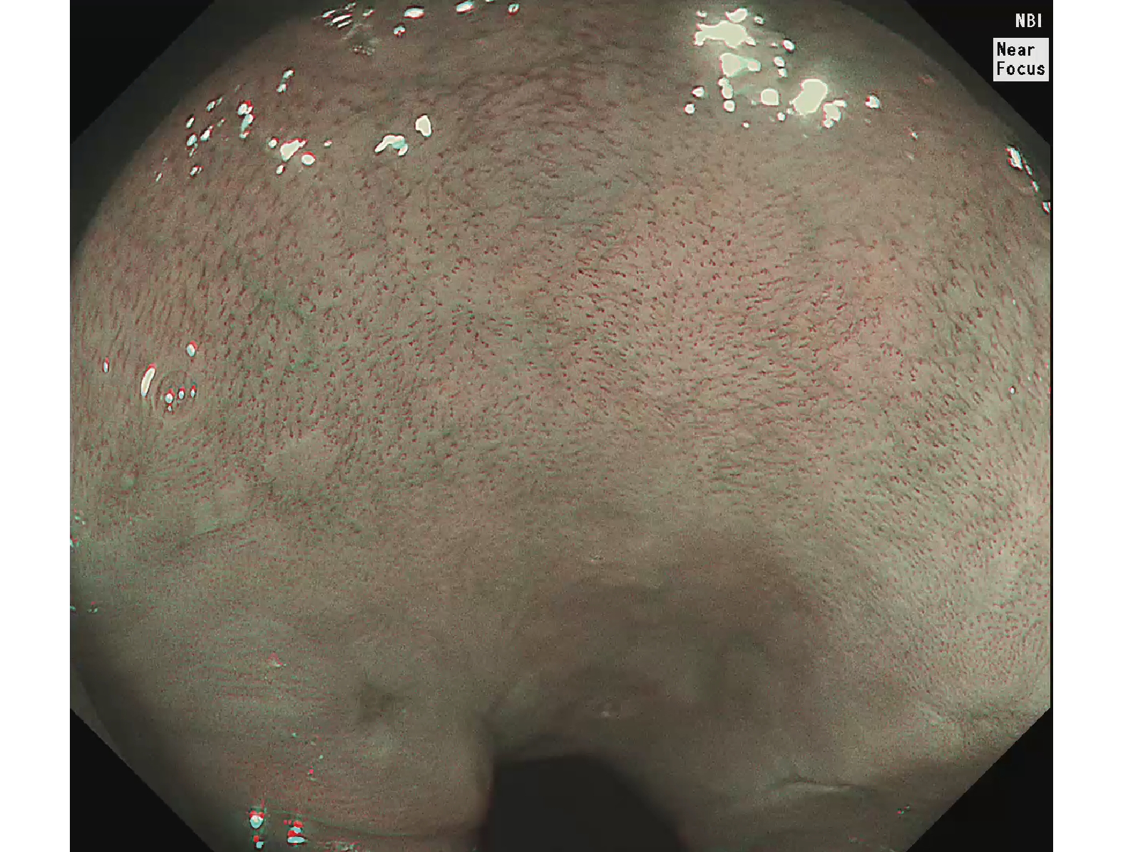
Figure 2. Full-size endoscopic image.
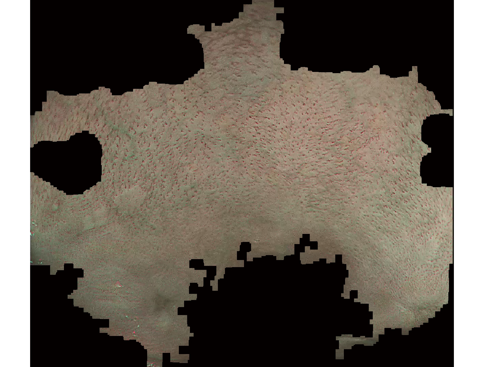
Figure 3. Region of the interest (ROI).
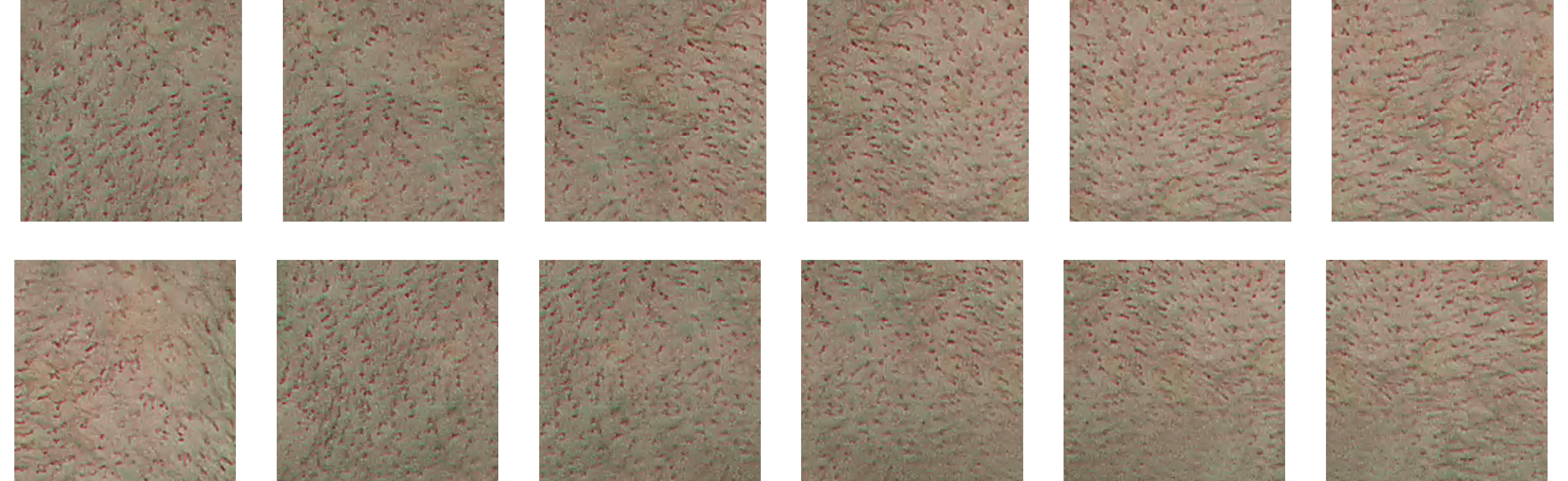
Figure 4. Image patches.
When training the NERD-CADS, we firstly extract the ROIs from the full-size endoscopic images (training samples) by the ROI-extraction algorithm. Then, we generate the image patches from the ROIs by the patch-generating algorithm. Next, we train the CNN using the image patches. After the training, the CNN can classify the image patches. When testing the NERD-CADS, we use the same algorithms to obtain the image patches from the full-size endoscopic images (test samples). Subsequently, we use the CNN to classify the image patches, and employ the majority voting method to summarize the final classification result from the classification results of the image patches. The experiment in our previous research [7] has shown that the classification accuracy of the NERD-CADS reaches 77.8%.
In this paper, we aim to improve the classification accuracy of the NERD-CADS by adding contrastive self-supervised learning as an additional component to the NERD-CADS (named NERD-CADS-CSSL). The contrastive self-supervised learning can learn the capability of extracting representations from image data by reducing the distance between the representations of two augmentations of the same image. This paper 1) combines the contrastive self-supervised learning with transfer learning, which employs massive public image data to train the CNN by the contrastive self-supervised learning; and 2) uses the endoscopic images to fine-tune the CNN. In this way, the capability of extracting representations (learned by the contrastive self-supervised learning) can be transferred to the downstream task (NERD diagnosis), which is able to improve the classification accuracy of the NERD-CADS.
We compare the NERD-CADS-CSSL with the NERD-CADS by subject-dependent and subject-independent experiments. In the subject-dependent experiment, the test images from the same group of subjects are used as the training images, and the test images that come from the unseen group of subjects cannot be used as the training images. Also, we perform the subject-independent experiment, where the images for training and test are from different groups of subjects. In the subject-independent experiment, we can verify whether the diagnosis systems can be generalized to the case where the test images are those from the unseen group of subjects. Moreover, we conduct ten-fold cross-validation in both experiments to verify the classification accuracy of the diagnosis systems. The experiment (to be presented in Section 4) will show that the NERD-CADS-CSSL can obtain a higher mean (80.6%) than the mean (77.8%) obtained by NERD-CADS. The contributions of this paper are summarized as follows.
1) We add the contrastive self-supervised learning as an additional component to the NERD-CADS, and investigate whether it can improve the classification accuracy of the NERD-CADS. The experiments show that the classification accuracy is indeed improved.
2) We transfer the capability of extracting representations (learned by the contrastive self-supervised learning) to the downstream task (NERD diagnosis), and investigate the transferability of the contrastive self-supervised learning. The experiments show that the contrastive self-supervised learning has good transferability.
3) We conduct the subject-dependent and the subject-independent experiments to investigate whether the diagnosis systems can be generalized to the case where the test images are those from the unseen group of subjects. The experiments show that the diagnosis systems have good generalization ability and consequently, it is practical to apply such systems to assist clinical diagnosis of NERD.
The rest of this paper is organized as follows: The background theory is introduced in Section 2. Section 3 describes the developed method of this paper. The experiments and results are demonstrated in Section 4. Section 5 draws the conclusion.
2. Background Theory
In this section, we will introduce contrastive self-supervised learning and transfer learning, which will be used to develop the method of this paper.
2.1. Contrastive Self-Supervised Learning
The contrastive self-supervised learning is a kind of self-supervised learning method. Using this method, a system can learn the capability of extracting representations from unlabeled images by itself. In most contrastive self-supervised learning methods [11-15], augmentations of the unlabeled images are generated first. The distances between the representations of different augmentations of the same image (called positive pairs) are then reduced, and the distances between the representations of augmentations of different images (called negative pairs) are finally increased. In this way, the capability of extracting representations from the unlabeled images can be learned. The experiments in [11-15] have shown that the capability of extracting representations learned by the contrastive self-supervised learning can be used for downstream tasks to improve the classification accuracy.
However, computing the distances between the negative pairs needs large memory. For improvement, the authors in [16] have proposed a contrastive self-supervised learning method, named bootstrap your own latent (BYOL), which only needs to reduce the distance between the positive pairs and does not need to use the negative pairs. The experiment in [16] has shown that BYOL can obtain higher classification accuracy than the contrastive self-supervised learning methods which require the positive and the negative pairs.
During the training, BYOL iteratively performs the following steps as shown in Figure 5, where the encoder  , the projector
  and the predictor
  have a set of weights and biases
  , while the encoder
  and the projector
  have a different set of weights and biases
  .
.

Figure 5. Architecture of bootstrap your own latent (BYOL).
At the first step, an unlabeled image  is randomly picked, and two augmentations
  and
and  from the unlabeled image
  are then generated. The augmentation methods include random cropping and resizing, left-right flip, color jittering, color dropping, Gaussian blurring and solarization. At the second step, the augmentations
  and
and  are fed, respectively, into the encoders
  and
and  . At the third step, representations
  and
and  are output, respectively, from the encoders
  , while
  is input into the projectors
  and
and  . The projectors
  and
and  are multi-layer perception (MLP) networks, and such networks consist of a fully connected layer followed by batch normalization [17], rectified linear unit (ReLU) [18] and a fully connected layer. At the fourth step, the projectors
  and
and  , respectively, output projections
  and
and  , and the projection
  is input into the predictor
  to produce the prediction
  , where the structure of the predictor
  is the same as the projectors
  and
and  . At the fifth step, the prediction
  and the projection
  are
are  -normalized by Equations (1) and (2). At the sixth step, the loss
  is calculated by the loss function Equation (3). At the seventh step, the augmentations
  and
and  are output, respectively, into encoders
  and
and  , and the third to the sixth steps are repeated to obtain the symmetrical loss
  (which is not described in Figure 5). Specifically, the prediction
  and the projection
  are
are  -normalized by Equations (4) and (5), and the symmetrical loss
  is calculated by the loss function Equation (6). At the eighth step, an optimizer is used to minimize Equation (7) with regard to
  (other than
  ) as described by “stop gradient” in Figure 5. At the ninth step, the exponential moving average [19] of
  Equation (8) is used to update
  .
.


where  is a decay rate.
After the training, BYOL only keeps the encoder  which can be used for downstream tasks to output representations of new images.
From the steps of BYOL described by Figure 5, it can be seen that the left network (  ,
,  and
and  ) extracts the representation of the augmentation of an image, and the right network (
  and
and  ) extracts the representation of another augmentation of the same image. Then, the optimizer tries to minimize the loss function which is the difference between the two representations. That is to say, BYOL tries to let the networks learn the capability of outputting the same representation for different augmentations of the same image. In other words, BYOL tries to let the networks learn the capability that, no matter what transformations are applied to the same image, the networks will output the same representation. In this way, the networks can learn the image invariance in a set of image transformations and consequently, output the representation that is not affected by the set of image transformations.
In the architecture of BYOL, it can be seen that there is an encoder followed by a projector to output the representation. The experiments in [11, 13-14] have shown that in comparison with the only use of the representation output from an encoder, higher classification accuracy can be obtained in the downstream task via the use of the representation output from an encoder followed by a projector. We conjecture the reason is that when adding a projector, the capability of extracting common features is learned by the encoder and the capability of extracting task-specific features is learned by the projector. Then, the encoder is used for the downstream task that only needs the capability of extracting common features exactly. Note that the capability of extracting task-specific features will be learned using another neural network for the downstream task. The experiment in [11] has shown that when adding a projector, the output from the encoder has much more information than the output from the projector for distinguishing whether image transformations are applied. This supports such a point of view.
Moreover, in the architecture of BYOL, it can be seen that a predictor follows the projector in the left network, and the structure of the predictor is the same as the projector. Meanwhile, it can be seen that the weights and biases of the right network are not updated by the gradients of the loss function, but by the exponential moving average [19] of the weights and biases of the left network, which can prevent the networks from converging to a collapsed constant solution [16]. However, the reason has not been explained thoroughly. Until now, the reason has still been an open question [20, 21].
2.2. Transfer Learning
The transfer learning [22] is a common method for training the CNN by using a dataset  to train the CNN for task A first. After the training, the CNN has learned the capability of extracting representations from the samples in the dataset
  . The representations contain common features and task-specific features, where the part for extracting the common features is kept and the part for extracting the task-specific features is restrained by using another dataset
  for task B. In this way, the capability of extracting the common features (learned from the first training) can be transferred to do task B, which can improve the performance of doing task B, especially when the dataset
  does not have a sufficient number of labeled training samples [22, 23].
3. Methods
This research aims to develop algorithms for automatic diagnosis of NERD in order to solve a classification problem of two classes: non-NERD and NERD. Ethical approval has been granted by the NHS Health Research Authority North West Research Ethics Committee (REC reference: 17/NW/0562) and informed consent has been obtained. In our previous paper [7], we have proposed the NERD-CADS that can classify the endoscopic images captured in the esophagus of both healthy people and NERD patients as introduced in Section 1. In this paper, we aim to improve the classification accuracy of the NERD-CADS.
We suppose that the capability of the CNN for extracting representations from image data may influence the classification accuracy. The conventional method trains the CNN to learn the capability of extracting representations by using the images and labels, which is a supervised learning method. Different from the supervised learning, the contrastive self-supervised learning can learn the capability of extracting representations by reducing the distance between the representations of two augmentations of the same image as introduced in Subsection 2.1. This may be more effective than the supervised learning. Therefore, we add the contrastive self-supervised learning as an additional component to the NERD-CADS, and investigate whether it can learn the capability of extracting representations better to improve the classification accuracy. This paper combines the contrastive self-supervised learning with the transfer learning, where massive public image data is employed to train the CNN (by the contrastive self-supervised learning) and the endoscopic images are used to fine-tune the CNN.
Before training the contrastive self-supervised learning algorithm, we first take the pretrained CNN (the pretrained Inception-ResNetV2 [24]) from our previous research [7]. We select the pretrained Inception-ResNetV2 [24] as the pretrained CNN because the pretrained Inception-ResNetV2 [24] obtains the highest classification accuracy in our previous research [7]. The pretrained CNN is trained using the ImageNet dataset [25]. Then, we keep the convolutional layers of the pretrained CNN only, which can be regarded as an encoder. Next, we conduct the following improvement for the NERD-CADS by combining the contrastive self-supervised learning with the transfer learning.
The illustration of the improvement for the NERD-CADS is shown in Figure 6, where the convolutional layers of the pretrained CNN  , the projector
  and the predictor
  have a set of weights and biases
  ; the convolutional layers of the pretrained CNN
  and the projector
  have a different set of weights and biases
  ; and the neural network
  has a different set of weights and biases
  . The method includes a contrastive self-supervised training phase followed by a supervised training phase and a test phase.

Figure 6. Illustration of the method.
During the contrastive self-supervised training phase, we iteratively perform the following steps. Firstly, we randomly pick an image  from the STL-10 dataset [26], and then generate two augmentations
  and
and  from the image
  . Each augmentation is generated by random cropping and resizing followed by a combination of randomly applying left-right flip, color jittering, color dropping, and Gaussian blurring from the image
  , which will be presented in Subsection 4.1 in detail [11, 16]. Secondly, we feed the augmentations
  and
and  , respectively, into the convolutional layers of the pretrained CNNs
  and
and  . Thirdly, representations
  and
and  output, respectively, from the convolutional layers of the pretrained CNNs
  and
and  , and are later input into the projectors
  and
and  . Fourthly, the projectors
  and
and  , respectively, output projections
  and
and  . Then, the projection
  is input into the predictor
  to produce the prediction
  . Fifthly, the prediction
  and the projection
  are
are  -normalized by Equations (1) and (2) in Subsection 2.1. Sixthly, we calculate the loss
  by Equation (3) in Subsection 2.1. Seventhly, we input the augmentations
  and
and  respectively into the convolutional layers of the pretrained CNNs
  and
and  and repeat the third to the sixth steps to obtain the symmetrical loss
  (that is not described in Figure 6). Specifically, the prediction
  and the projection
  are
are  -normalized by Equations (4) and (5) in Subsection 2.1, and the symmetrical loss
  is calculated by Equation (6) in Subsection 2.1. Eighthly, we use an optimizer to minimize Equation (7) in Subsection 2.1 with regard to
  only, but not
  , as described by “stop gradient” in Figure 6. Ninthly, we use the exponential moving average [19] of
  (Equation (8) in Subsection 2.1) to update
  . In this way, the networks can learn the image invariance in a set of image transformations and consequently, can output a representation that is not affected by the set of image transformations (refer to Subsection 2.1). After the training, we only keep the convolutional layers of the pretrained CNN
  for the following task.
During the supervised training phase, we firstly extract the ROIs from the full-size endoscopic images (training samples) by the ROI-extraction algorithm [7] in Figure 1. Then, we generate the image patches from the ROIs by the patch-generating algorithm [7] in Figure 1. Next, we iteratively perform the following steps. Firstly, we pick an image patch  , and feed it into the convolutional layers of the pretrained CNN
  . Secondly, the representation
  (the output from the convolutional layers of the pretrained CNN
  ) is input into the neural network
  . The neural network
  consists of a fully connected layer followed by a softmax function. Thirdly, the neural network
  outputs a predicted label
  . The predicted label
  has two elements
  and
and  that represent the possibility of the image patch
  falling into non-NERD and NERD, respectively. The true label
  is encoded by one-hot. That is, if the true label
  is non-NERD, then
  and
and  ; if the true label
  is NERD, then
  and
and  . Then, we calculate the cross-entropy loss
  by Equation (9). Fourthly, we use an optimizer to minimize Equation (9) with regard to
  and
and  . In this way, the image invariance in a set of image transformations learned by the convolutional layers of the pretrained CNN
  can be transferred to do the classification of the image patches. After the training, we keep the convolutional layers of the pretrained CNN
  and the neural network
  for the test.

During the test phase, we firstly extract the ROIs from the full-size endoscopic images (test samples) by the ROI-extraction algorithm [7] in Figure 1. Then, we generate the image patches from the ROIs by the patch-generating algorithm [7] in Figure 1. Next, we iteratively perform the following steps. Firstly, we pick an image patch  , and feed it into the convolutional layers of the pretrained CNN
  . Secondly, a representation
  output from the convolutional layers of the pretrained CNN
  is input into the neural network
  . Thirdly, the neural network
  outputs a predicted label
  . Then, we record the predicted label
  of the image patch
  for the calculation of the classification accuracy. After all the image patches are predicted, we check all the predicted labels with the corresponding true labels and calculate the classification accuracy on the image level. Next, we calculate the predicted classes on the subject level by the majority voting [7] in Figure 1. The majority voting [7] is that, if more than 50% of the image patches from a subject are predicted as one class, we predict this subject as this class. Then, we check all the predicted classes of subjects with the corresponding true classes and calculate the classification accuracy on the subject level.
4. Experiments and Results
We compare the classification accuracy (defined as Equation (10)) of the NERD-CADS with that of the NERD-CADS-CSSL by the subject-dependent and the subject-independent experiments as introduced in Section 1. Meanwhile, we conduct ten-fold cross-validation in both experiments to verify the classification accuracy. The same dataset in our previous paper [7] is used for the experiments. In the subject-dependent experiment, we use 1394 full-size endoscopic images from 50 subjects, where 554 full-size endoscopic images from 21 subjects are labeled as “positive” (NERD patients), and 840 full-size endoscopic images from 29 subjects are labeled as “negative” (healthy people). In the subject-independent experiment, we use 556 full-size endoscopic images from a different group of subjects (18 subjects), where 229 full-size endoscopic images from 6 subjects are labeled as “positive” (NERD patients), and 327 full-size endoscopic images from 12 subjects are labeled as “negative” (healthy people).

where  ,
,  ,
,  , and
, and  respectively denote the number of true-positive, false-positive, true-negative, and false-negative classification results [27].
4.1. Implementation Details
Augmentation Methods
The augmentation policy consists of random cropping and resizing followed by a combination of randomly applying left-right flip, color jittering, color dropping, and Gaussian blurring [11, 16]. The possibility of applying each augmentation method is listed in Table 1. The details of the augmentation methods are given as follows:
• Random cropping and resizing: The image is randomly cropped by a window from 8% to 100% of the original image size and from 3/4 to 4/3 of the original image aspect ratio. Then, the cropped image is resized to 299 × 299 pixels by bilinear interpolation.
• Left-right flip: The image is flipped in the left-right direction.
• Color jittering: The brightness, contrast, saturation, and hue of the image are changed to random extent within a range. The range of the changed brightness is 20% to 180% of the original image brightness. The range of the changed contrast is 20% to 180% of the original image contrast. The range of the changed saturation is 20% to 180% of the original image saturation. The range of the changed hue is 80% to 120% of the original image hue.
• Color dropping: The image is converted to grayscale. Given that the red, green, and blue channels of the image are  ,
,  , and
, and  , then the grayscale image is
  .
.
• Gaussian blurring: The image is blurred by a Gaussian kernel with the standard deviation of 1.5, and the kernel size is 30 × 30.
Table 1. The possibility of applying each augmentation method.
| Augmentation Methods | Possibility |
| Random Cropping and Resizing | 1.0 |
| Left-Right Flip | 0.5 |
| Color Jittering | 0.8 |
| Color Dropping | 0.2 |
| Gaussian Blurring | 0.1 |
Parameters and Configurations
The parameters and configurations of the method in this paper are listed in Table 2, which are determined by trial and error.
Table 2. Parameters and configurations.
| Contrastive Self-Supervised Training Phase |  , ,  |
Structure: Inception-ResNetV2 [24]. |
Input size: 299  299 299  3. 3. |
||
| Output size: 1536. | ||
 , ,  |
Structure: a fully connected layer followed by batch normalization [17], | |
| ReLU [18], and a fully connected layer. | ||
| The first fully connected layer: input size: 1536; output size: 4096. | ||
| The second fully connected layer: input size: 4096; output size: 256. | ||
 |
Structure: a fully connected layer followed by batch normalization [17], | |
| ReLU [18], and a fully connected layer. | ||
| The first fully connected layer: input size: 256; output size: 4096. | ||
| The second fully connected layer: input size: 4096; output size: 256. | ||
 |
0.99. | |
| Batch Size | 128. | |
| Optimizer | Stochastic gradient descent with momentum. | |
| Supervised Training Phase |  |
Structure: a fully connected layer followed by a softmax function. |
| Input size: 1536. | ||
| Output size: 2. | ||
| Batch Size | 128. | |
| Optimizer | Stochastic gradient descent with momentum. |
4.2. Subject-Dependent Experiment
In the subject-dependent experiment, we randomly divide the 1394 full-size endoscopic images from 50 subjects into two parts. One part contains approximately 70% of the full-size endoscopic images that are used for the ten-fold cross-validation, and another part contains approximately 30% of the full-size endoscopic images that are used for the test. Then, the first part is divided into ten folds. Each fold contains approximately the same number of the images. The scheme for dividing the images is illustrated in Figure 7. Each fold consists of 10% images of each subject. After the images are divided, we use the images of the fold  as the validation samples and the images of the remaining nine folds as the training samples.
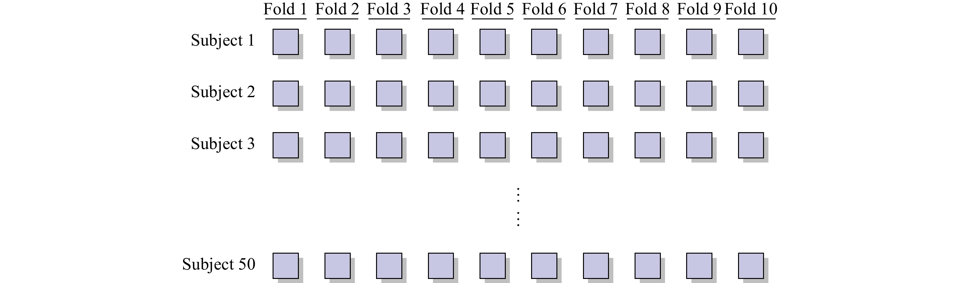
Figure 7. Scheme of the division.
As the result of the experiment plan, each fold consists of a proportion of the images of each subject. Thus, it is a subject-dependent classification. Consequently, we only perform the classification on the image level in the subject-dependent experiment.
Tables 3 and 4 show the classification accuracy on the image level in the training and test of the NERD-CADS (from our previous research [7]) and the NERD-CADS-CSSL in the subject-dependent experiment.
Table 3. Classification accuracy on image level in training of the NERD-CADS and the NERD-CADS-CSSL in the subject-dependent experiment.
| Fold | Classification Accuracy on Image Level in Training | |
| NERD-CADS | NERD-CADS-CSSL | |
| * Mean, STD, Best, and Worst respectively denote mean, standard deviation, the best, and the worst of classification accuracy from ten-fold cross-validation. | ||
| 1 | 99.1% | 99.3% |
| 2 | 99.2% | 99.3% |
| 3 | 98.2% | 99.2% |
| 4 | 98.4% | 99.7% |
| 5 | 99.3% | 99.7% |
| 6 | 99.7% | 99.4% |
| 7 | 98.5% | 99.2% |
| 8 | 99.5% | 99.3% |
| 9 | 99.9% | 99.9% |
| 10 | 99.9% | 100.0% |
| Mean | 99.2% | 99.5% |
| STD | 0.6% | 0.3% |
| Best | 99.9% | 100.0% |
| Worst | 98.2% | 99.2% |
Table 4. Classification accuracy on image level in test of the NERD-CADS and the NERD-CADS-CSSL in the subject-dependent experiment.
| Fold | Classification Accuracy on Image Level in Test | |
| NERD-CADS | NERD-CADS-CSSL | |
| * Mean, STD, Best, and Worst respectively denote mean, standard deviation, the best, and the worst of classification accuracy from ten-fold cross-validation. | ||
| 1 | 82.7% | 91.3% |
| 2 | 85.0% | 89.0% |
| 3 | 83.5% | 88.6% |
| 4 | 84.1% | 94.1% |
| 5 | 86.6% | 91.8% |
| 6 | 91.3% | 96.3% |
| 7 | 86.5% | 95.1% |
| 8 | 87.5% | 93.5% |
| 9 | 85.7% | 91.3% |
| 10 | 97.4% | 93.8% |
| Mean | 87.0% | 92.5% |
| STD | 4.1% | 2.4% |
| Best | 97.4% | 96.3% |
| Worst | 82.7% | 88.6% |
In Table 3, compared with the NERD-CADS, it can be seen that the NERD-CADS-CSSL obtains a higher mean of ten-fold classification accuracy on the image level in training. The increase is 0.3% (99.5% − 99.2%). Moreover, compared with the NERD-CADS, it can be seen that the NERD-CADS-CSSL has a lower standard deviation of ten-fold classification accuracy on the image level in training. The decrease is 0.3% (0.6% − 0.3%), which means that the classification accuracy is more stable. In Table 4, compared with the NERD-CADS, it can be seen that the NERD-CADS-CSSL obtains a higher mean of ten-fold classification accuracy on the image level in test. The increase is 5.5% (92.5% − 87.0%). Moreover, compared with the NERD-CADS, it can be seen that the NERD-CADS-CSSL has a lower standard deviation of ten-fold classification accuracy on the image level in test. The decrease is 1.7% (4.1% − 2.4%), which means that the classification accuracy is more stable.
The results show that the capability of extracting the common features learned by the contrastive self-supervised learning can be transferred to the downstream task (NERD diagnosis). This improves the classification accuracy of the downstream task (NERD diagnosis), demonstrating that the contrastive self-supervised learning has good transferability.
4.3. Subject-Independent Experiment
In the subject-independent experiment, we test the NERD-CADS and the NERD-CADS-CSSL that have been trained from the subject-dependent experiment. We divide the 556 full-size endoscopic images from a different group of subjects (18 subjects) by the subject. Then, we use the images as the test samples. Thus, the training and the test samples are from different groups of subjects. Consequently, it is the subject-independent classification. We perform the classification on the image level and subject level in the subject-independent experiment.
Tables 5 and 6 show the classification accuracy on the image level and subject level in test of the NERD-CADS (from our previous research [7]) and the NERD-CADS-CSSL in the subject-independent experiment.
Table 5. Classification accuracy on image level in test of the NERD-CADS and the NERD-CADS-CSSL in the subject-independent experiment.
| Fold | Classification Accuracy on Image Level in Test | |
| NERD-CADS | NERD-CADS-CSSL | |
| * Mean, STD, Best, and Worst respectively denote mean, standard deviation, the best, and the worst of classification accuracy from ten-fold cross-validation. | ||
| 1 | 70.4% | 75.0% |
| 2 | 72.1% | 73.4% |
| 3 | 73.6% | 74.1% |
| 4 | 66.7% | 74.6% |
| 5 | 67.6% | 72.3% |
| 6 | 69.3% | 71.9% |
| 7 | 70.8% | 72.2% |
| 8 | 70.7% | 75.3% |
| 9 | 71.5% | 73.7% |
| 10 | 67.4% | 76.5% |
| Mean | 70.0% | 73.9% |
| STD | 2.1% | 1.4% |
| Best | 73.6% | 76.5% |
| Worst | 66.7% | 71.9% |
Table 6. Classification accuracy on subject level in test of the NERD-CADS and the NERD-CADS-CSSL in the subject-independent experiment.
| Fold | Classification Accuracy on Subject Level in Test | |
| NERD-CADS | NERD-CADS-CSSL | |
| * Mean, STD, Best, and Worst respectively denote mean, standard deviation, the best, and the worst of classification accuracy from ten-fold cross-validation. | ||
| 1 | 88.9% | 88.9% |
| 2 | 77.8% | 88.9% |
| 3 | 83.3% | 77.8% |
| 4 | 77.8% | 77.8% |
| 5 | 72.2% | 83.3% |
| 6 | 77.8% | 88.9% |
| 7 | 72.2% | 83.3% |
| 8 | 77.8% | 72.2% |
| 9 | 77.8% | 66.7% |
| 10 | 72.2% | 77.8% |
| Mean | 77.8% | 80.6% |
| STD | 5.0% | 7.1% |
| Best | 88.9% | 88.9% |
| Worst | 72.2% | 66.7% |
In Table 5, it can be seen that the NERD-CADS-CSSL obtains a higher mean of ten-fold classification accuracy on the image level in test than the NERD-CADS. The increase is 3.9% (73.9% − 70.0%). Moreover, it can be seen that the NERD-CADS-CSSL has a lower standard deviation of ten-fold classification accuracy on the image level in test than the NERD-CADS. The decrease is 0.7% (2.1% − 1.4%), which means that the classification accuracy is more stable. In Table 6, it can be seen that the NERD-CADS-CSSL obtains a higher mean of ten-fold classification accuracy on the subject level in test than the NERD-CADS. The increase is 2.8% (80.6% − 77.8%). However, it can be seen that the NERD-CADS-CSSL has a higher standard deviation of ten-fold classification accuracy on subject level in test than the NERD-CADS. The increase is 2.1% (7.1% − 5.0%), which means the classification accuracy is less stable.
The results show that the contrastive self-supervised learning can improve the classification accuracy of the NERD-CADS. Moreover, the results demonstrate that the NERD-CADS and the NERD-CADS-CSSL can be generalized to handle the test images that come from the unseen group of subjects.
5. Conclusion
This paper has added the contrastive self-supervised learning as an additional component to the NERD-CADS to investigate whether it can improve the classification accuracy of the NERD-CADS. We have combined the contrastive self-supervised learning with the transfer learning. This means that massive public image data has been employed to train the CNN by the contrastive self-supervised learning first, and then the endoscopic images have been used to fine-tune the CNN for the downstream task (NERD diagnosis). We have compared the NERD-CADS with the NERD-CADS-CSSL in the subject-dependent and the subject-independent experiments. Moreover, we have conducted ten-fold cross-validation in both experiments to verify the classification accuracy. The experiments have shown that the contrastive self-supervised learning can improve the classification accuracy of the NERD-CADS. Meanwhile, the experiments have shown that the capability of extracting the common features learned by the contrastive self-supervised learning can be transferred to the downstream task (NERD diagnosis). This has improved the classification accuracy of the downstream task (NERD diagnosis), and demonstrated that the contrastive self-supervised learning has good transferability. Moreover, the experiments have shown that the NERD-CADS and the NERD-CADS-CSSL can be generalized to handle the endoscopic images (test samples) that come from the unseen group of subjects.
Author Contributions: Junkai Liao: conceptualization, methodology, software, investigation, writing - original draft preparation. Hak-Keung Lam: writing - review and editing, supervision, project administration. Shraddha Gulati: resources, data curation. Bu Hayee: resources, project administration. All authors have read and agreed to the published version of the manuscript.
Funding: This research was partly supported by King's College London and China Scholarship Council.
Data Availability Statement: Not applicable.
Conflicts of Interest: The authors declare no conflict of interest.
References
- Martinez, S.D.; Malagon, I.B.; Garewal, H.S.; et al. Non-erosive reflux disease (NERD) - acid reflux and symptom patterns. Aliment. Pharmacol. Ther., 2003, 17: 537−545.
- Narayani, R.I.; Burton, M.P.; Young, G.S. Utility of esophageal biopsy in the diagnosis of nonerosive reflux disease. Dis. Esophagus, 2003, 16: 187−192.
- Modlin, I.M.; Hunt, R.H.; Malfertheiner, P.; et al. Diagnosis and management of non-erosive reflux disease - the vevey NERD consensus group. Digestion, 2009, 80: 74−88.
- Chen, C.L.; Hsu, P.I. Current advances in the diagnosis and treatment of nonerosive reflux disease. Gastroenterol. Res. Pract., 2013, 2013: 653989.
- Khan, M.Q.; Alaraj, A.; Alsohaibani, F.; et al. Diagnostic utility of impedance-pH monitoring in refractory non-erosive reflux disease. J. Neurogastroenterol. Motil., 2014, 20: 497−505.
- Barrett, C.; Choksi, Y.; Vaezi, M.F. Mucosal impedance: A new approach to diagnosing gastroesophageal reflux disease and eosinophilic esophagitis. Curr. Gastroenterol. Rep., 2018, 20: 33.
- Liao, J.K.; Lam, H.K.; Jia, G.; et al. A case study on computer-aided diagnosis of nonerosive reflux disease using deep learning techniques. Neurocomputing, 2021, 445: 149−166.
- Huang, C.R.; Chen, Y.T.; Chen, W.Y.; et al. Gastroesophageal reflux disease diagnosis using hierarchical heterogeneous descriptor fusion support vector machine. IEEE Trans. Biomed. Eng., 2016, 63: 588−599.
- Fass, R.; Fennerty, B.M.; Vakil, N. Nonerosive reflux disease - current concepts and dilemmas. Am. J. Gastroenterol., 2001, 96: 303−314.
- Fass, R. Erosive esophagitis and nonerosive reflux disease (NERD): Comparison of epidemiologic, physiologic, and therapeutic characteristics. J. Clin. Gastroenterol., 2007, 41: 131−137.
- Chen, T.; Kornblith, S.; Norouzi, M.; et al. A simple framework for contrastive learning of visual representations. In Proceedings of the 37th International Conference on Machine Learning, 13–18 July 2020; JMLR.org, 2020; pp. 1597–1607.
- Chen, T.; Kornblith, S.; Swersky, K.; et al. Big self-supervised models are strong semi-supervised learners. In Proceedings of the 34th International Conference on Neural Information Processing Systems, Vancouver, Canada, 6–12 December 2020; Curran Associates Inc.: Red Hook, 2020; pp. 22243–22255.
- He, K.M.; Fan, H.Q.; Wu, Y.X.; et al. Momentum contrast for unsupervised visual representation learning. In Proceedings of 2020 IEEE/CVF Conference on Computer Vision and Pattern Recognition, Seattle, WA, USA, 13–19 June 2020; IEEE: New York, 2020; pp. 9726–9735. doi: 10.1109/CVPR42600.2020.00975
- Chen, X.L.; Fan, H.Q.; Girshick, R.; et al. Improved baselines with momentum contrastive learning. arXiv: 2003.04297, 2020. doi: 10.48550/arXiv.2003.04297
- Chen, X.L.; Xie, S.N.; He, K.M. An empirical study of training self-supervised vision transformers. In Proceedings of 2021 IEEE/CVF International Conference on Computer Vision, Montreal, Canada, 10–17 October 2021; IEEE: New York, 2021; pp. 9620–9629. doi: 10.1109/ICCV48922.2021.00950
- Grill, J.B.; Strub, F.; Altché, F.; et al. Bootstrap your own latent a new approach to self-supervised learning. In Proceedings of the 34th International Conference on Neural Information Processing Systems, Vancouver, Canada, 6–12 December 2020; Curran Associates Inc.: Red Hook, 2020; pp. 21271–21284.
- Ioffe, S.; Szegedy, C. Batch normalization: Accelerating deep network training by reducing internal covariate shift. In Proceedings of the 32nd International Conference on International Conference on Machine Learning, Lille, France, 6–11 July 2015; JMLR.org, 2015; pp. 448–456.
- Nair, V.; Hinton, G.E. Rectified linear units improve restricted Boltzmann machines. In Proceedings of the 27th International Conference on International Conference on Machine Learning, Haifa, Israel, 21–24 June 2010; Omnipress, 2010; pp. 807–814.
- Lillicrap, T.P.; Hunt, J.J.; Pritzel, A.; et al. Continuous control with deep reinforcement learning. In Proceedings of the 4th International Conference on Learning Representations, San Juan, USA, 2–4 May 2016; ICLR: Ithaca, 2015. doi: 10.48550/arXiv.1509.02971
- Tian, Y.D.; Yu, L.T.; Chen, X.L.; et al. Understanding self-supervised learning with dual deep networks. arXiv: 2010.00578v1, 2020. doi: 10.48550/arXiv.2010.00578
- Richemond, P.H.; Grill, J.B.; Altché, F.; et al. BYOL works even without batch statistics. arXiv: 2010.10241, 2020. doi: 10.48550/arXiv.2010.10241
- Pan, S.J.; Yang, Q. A survey on transfer learning. IEEE Trans. Knowl. Data Eng., 2010, 22: 1345−1359.
- Torrey, L.; Shavlik, J. Transfer learning. In Handbook of Research on Machine Learning Applications and Trends: Algorithms, Methods, and Techniques; Olivas, E.S; Guerrero, J.D.M.; Martinez-Sober, M.; et al., Eds.; IGI Global: Hershey, 2010; pp. 242–264. doi: 10.4018/978-1-60566-766-9.ch011
- Szegedy, C.; Ioffe, S.; Vanhoucke, V.; et al. Inception-v4, inception-ResNet and the impact of residual connections on learning. In Proceedings of the Thirty-First AAAI Conference on Artificial Intelligence, San Francisco, USA, 4–9 February 2017; AAAI: Palo Alto, 2017; pp. 4278–4284.
- Deng, J.; Dong, W.; Socher, R.; et al. ImageNet: A large-scale hierarchical image database. In Proceedings of the 2009 IEEE Conference on Computer Vision and Pattern Recognition, Miami, USA, 20–25 June 2009; IEEE: New York, 2009; pp. 248–255. doi: 10.1109/CVPR.2009.5206848
- Coates, A.; Ng, A.; Lee, H. An analysis of single-layer networks in unsupervised feature learning. In Proceedings of the 14th International Conference on Artificial Intelligence and Statistics, Fort Lauderdale, USA, 11–13 April 2011; PMLR, 2011; pp. 215–223.
- Metz, C.E. Basic principles of ROC analysis. Semin. Nucl. Med., 1978, 8: 283−298.