

Downloads
Download


This work is licensed under a Creative Commons Attribution 4.0 International License.
Article
Dynamic Scheduling for Large-Scale Flexible Job Shop Based on Noisy DDQN
Tingjuan Zheng 1,2, Yongbing Zhou 1, Mingzhu Hu 1, and Jian Zhang 1,*
1 Institute of Advanced Design and Manufacturing, School of Mechanical Engineering Southwest Jiaotong University, Chengdu 610031, China
2 Guizhou Aerospace Electric Co., Ltd., Guiyang 550009, China
* Correspondence: Jerrysmail@263.net
Received: 3 July 2023
Accepted: 8 October 2023
Published: 21 December 2023
Abstract: The large-scale flexible job shop dynamic scheduling problem (LSFJSDSP) has a more complex solution space than the original job shop problem because of the increase in the number of jobs and machines, which makes the traditional solution algorithm unable to meet the actual production requirements in terms of the solution quality and time. To address this problem, we develop a dynamic scheduling model of a large-scale flexible job shop based on noisynet-double deep Q-networks (N-DDQNs), which takes the minimum expected completion time as the optimization objective and thoroughly takes into account the two dynamic factors (the new job arrival and the stochastic processing time). Firstly, a Markov decision process model is constructed for dynamic scheduling of a large-scale flexible workshop, and the corresponding reasonable state space, action space and reward function are designed. To address the problems (of solution stability and unsatisfactory scheduling strategy selection) in the conventional exploration method of DDQNs, learnable noise parameters are added to the DDQNs to create the N-DDQN algorithm framework, where the uncertainty weight is added. Secondly, the learnable noise parameters are added to the DDQNs to form the N-DDQN algorithm framework, and the uncertainty weight is added to realize automatic exploration. Hence, the issue is solved that the traditional DDQN exploration method may result in unsatisfactory solution stability and scheduling strategy selection. The proposed method, which has significant flexibility and efficacy, is demonstrated (by experimental findings) to be superior to the conventional method based on compound scheduling rules in tackling large-scale flexible job shop dynamic scheduling problems.
Keywords:
large-scale flexible job shop dynamic scheduling new job arrival stochastic processing time deep reinforcement learning1. Introduction
Flexible job shop scheduling problems (FJSSPs) have been widely found in semiconductor manufacturing, automobile assembly, machinery manufacturing and other fields due to their flexibility with the actual production mode of the workshop [1]. The FJSSP is frequently extended to a large-scale flexible job shop scheduling problem (LSFJSP) in the actual production of complex parts, such as aviation equipment, rail transit equipment, and weapon equipment, due to the increasing numbers of parts and machines. Due to the influence of a large number of dynamic interference events, such as the machine breakdown, change of delivery time, new job arrival and stochastic processing time, etc., a typical large-scale flexible job shop dynamic scheduling problem (LSFJSDSP) is further formed, which has an exponentially increasing number of feasible solutions as the problem size grows. The search solution space has gradually become exceedingly complex due to the abundance of locally optimal solutions, making it a research hotspot and an industry focus.
The order-based production mode has become a common production mode in the manufacturing industry over the past few years as a result of the continued development of network technology and the manufacturing sector. As a result, the arrival of new workpieces has become an essential disturbance factor in this production mode [2−4]. The fluctuation of processing hours will be caused by the replacement of tools or tooling, the alteration of cutting parameters, the irregular maintenance of equipment, and the operational expertise of workers during the production process. Hence, the stochastic processing time has also become a significant disturbance factor affecting production efficiency, and has become a research topic for dynamic scheduling in recent years [5−8]. Actual production may experience two different dynamic disruptions at once. Therefore, it is more appropriate for the actual production environment to take into account the two disturbance aspects of the new workpiece arrival and the erratic working hours.
The workshop scheduling problem is the subject of numerous optimization proposals [9], but the scale of the solutions is typically not large. Although large-scale scheduling problems cannot be directly solved by many traditional optimization techniques due to both efficiency and quality issues, such problems can currently be resolved by problem-based decomposition approaches that include the decomposition method based on the model structure, time, workpiece and machine. For example, Van et al. [10] used the D-W algorithm to solve the machine scheduling problem, and proved that the method can effectively decompose the model of complex problems to simplify the model requirements. Liu et al. [11] iteratively decomposed the original large-scale scheduling problem into several sub-problems by resorting to the rolling horizon decomposition method and the prediction mechanism, and proposed an adaptive genetic algorithm to optimize each sub-problem.
In general, when addressing complex flexible job shop scheduling issues, the problem-based decomposition strategy described above has achieved some positive results, although there are still certain limitations that can be listed as follows. 1) It is difficult to guarantee the quality and speed of the solution when this method divides the large-scale FJSSP into smaller sub-problems because additional constraints will be generated for each sub-problem. 2) Most decomposition algorithms are complex and do not adequately account for dynamic infection factors (like the arrival of new jobs and random working hours in the actual process), making them unsuitable to be used in actual production. Therefore, it is crucial to research more effective scheduling optimization methods for resolving LSFJSDSPs.
Deep reinforcement learning (DRL) has recently emerged as a more advantageous approach for resolving scheduling problems with multiple interference factors and dynamic interference factors due to its ability to achieve real-time scheduling optimization of the production line. For instance, Luo et al. [12] proposed an online rescheduling framework for a two-level deep Q-network with the two practical objectives (of the total weighted delay rate and the average machine utilization rate) optimized. Luo [13] proposed a deep Q-network and six rules to solve the dynamic FJSSP with new order insertion in continuous production. Gui et al. [14] proposed a Markov decision process with compound scheduling actions, which converts DFJSP into RL tasks and trains the policy network (based on the deep deterministic policy gradient algorithm) to complete the weight training.
To solve the problem that reinforcement learning is limited by scale, a deep neural network is added to the reinforcement learning to fit Q values. For example, Waschneck et al. [15] designed some DQN-based collaborative agents for job shops. Each agent is responsible for optimizing the scheduling rules (of a work center and the global reward) while monitoring the behavior of other agents. For LSFJSPs, Song et al. [16] proposed a new DRL method to solve the difficult problem of one-to-many relationships existing in complex shop scheduling processes (in terms of decision-making and state representation), and verified its effectiveness in large-scale cases. Park et al. [17] proposed a semiconductor packaging device scheduling method based on deep reinforcement learning, and introduced a new state representation to effectively adapt to changes in the number of available machines and production demands.
Note that the existing research on algorithms for LSFJSPs pays little attention to practical dynamic scheduling, and has limitations of poor algorithm stability and low solution accuracy. Therefore, this paper systematically studies the LSFJSP based on the new job arrival and stochastic processing time, and designs pertinent dynamic scheduling methods based on the DRL. The main contributions are given as follows. 1) The FJSSP is extended to an FJSP based on the new job arrival and random working hours, and a real-time scheduling framework based on the N-DDQN algorithm is constructed to solve the dynamic scheduling model of the large-scale flexible job shop. 2) The state feature and the sensitive action set of the LSFJSP are designed, and the round and single-step hybrid reward mechanism is established to ensure the feasibility of the deep reinforcement learning framework and solve the scheduling problem. 3) The noisynet and the DDQN are combined to solve dynamic FJSSPs, where a set of learnable noise parameters is added to double-DQN networks, and weights are introduced into uncertainties to realize automatic exploration.
The remainder of the paper is organized as follows. Section 2 introduces the description and mathematical model of LSFJSDSPs based on the new job arrival and stochastic processing time. The noisy DDQN algorithm for flexible job shop dynamic scheduling is introduced in Section 3, which includes the design process of the state characteristics, action set and reward function. Section 4 completes the experimental design and analysis. Finally, the conclusion and future perspectives are drawn.
2. Problem Description and Mathematical Model
2.1. Description of the Problem
Compared with conventional flexible job-shop scheduling issues, LSFJSPs are more prone to interruption from new order insertion due to larger scales, more production resources, and higher volumes of workpieces. The ambiguity of working hours is one of the most frequent factors that reduces the actual output. Several variables, such as the arrival time of materials, the rate at which fixtures must be replaced, the modifications of industry parameters, the equipment breakdown or repair, the operator skill level, and the fatigue, all contribute to the unpredictable nature of the processing time. It can be seen that the new job arrival and time uncertainty are common disturbances in actual production, and in a production execution process, the two disturbances may exist simultaneously. Therefore, a large-scale flexible job shop dynamic scheduling mathematical model is established based on the expected completion time.
Based on the new job arrival and stochastic processing time, the large-scale dynamic scheduling problem of the flexible job shop needs to allocate  initial workpieces (
  , and
, and  workpieces
  to the machine tool according to the process route of the workpiece to achieve the optimization of the scheduling goal. The set of
  workpieces to be processed consists of the initial set of workpieces and the set of inserted workpieces, where each workpiece has Pi processing procedures. All processes in the initial workpiece set can be processed at time zero, as illustrated in Figure 1, and all processes are defined by normally distributed random variables for their working times. However, the inserted workpiece cannot be treated until it reaches time point Ai.
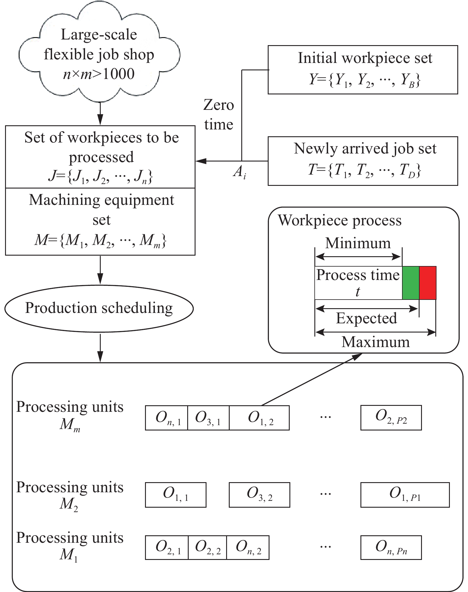
Figure 1. Schematic diagram of large-scale flexible job shop scheduling problem-based on new job arrival and stochastic processing time.
The LSFJSP model should be established with the following constraints since it is expanded from the static scheduling problem of the large-scale flexible job shop by considering two uncertain interference factors (i.e. the new job arrival and stochastic processing time).
1) The processing preparation time is not considered separately in the processing time.
2) The initial workpieces set can be processed at zero time, and the start time of all processes in the inserted workpieces set shall not be earlier than the arrival time of the new job.
3) The working hours of the process are random variables subject to normal distributions.
4) Each machine tool can only run one process at a certain time. Once each process starts, it shall not be interrupted.
5) The next process of the workpiece can only be processed after the completion of the previous process.
6) At the same time, each process of the workpiece is processed by one machine only.
7) The machine tool can be started at zero time, and the workpiece can be processed at zero time.
8) The processes of different workpieces do not have sequential constraints.
9) The product of the number of pieces and the number of machines shall not be less than 1000.
2.2. Mathematical Model
Aiming at the static scheduling problem of large-scale flexible job shops, the minimum completion time is taken as the optimization objective. The relevant variables are defined in Table 1 to establish a mathematical model. Based on the above assumptions, the static scheduling mathematical model can be obtained as follows. Optimization objectives:

Constraint conditions:


Here, Equation (1) represents the minimum maximum completion time; Equation (2) indicates that the start time and the processing time of each process on the  th machine are non-negative; Equation (3) means that each process can only be processed on one machine; Equation (4) means that each machine can only run one process at the same time; Equation (5) indicates that the next process can be processed only after the previous process is completed; Equation (6) is the large-scale qualification condition; and Equation (7) is the value range of the decision variable.
Table 1. Table of symbols and definitions
| Symbol | Description |
| J | Set of workpieces to be processed |
| n | Number of workpieces to be processed |
| M | Machine set |
| m | Number of machines |
 |
The number of processes of the  workpiece workpiece |
| i | Workpiece index (i = {1, 2, ···, n}) |
| j | Workpiece process index (j = {1, 2, ···,  }) }) |
| k | Machine index (k = {1, 2, ···, m}) |
 |
The  process of the process of the  workpiece workpiece |
 |
The processing time of process  on the machine on the machine  |
 |
The start processing time of process  on the machine on the machine  |
 |
The completion time of the job i |
 |
The decision variable determines whether the process is processed on  |
Based on the static scheduling problem, a large-scale flexible job shop dynamic scheduling model is created with the same optimization objective of minimizing the expected completion time. The start time and the end time of the procedure are also random variables because the processing time is a random variable. We simulate the expected completion time through the Monte Carlo sampling method, and the expected completion time can be expressed as the following equation.

Here,  represents the maximum completion time; Z is the Monte Carlo sampling frequency; and z is the Monte Carlo sampling frequency index. Although the processing time and the completion time in a dynamic scheduling problem are uncertain, the processing method for each workpiece is known. The limitations between the process and the machine tool should be satisfied, and the following constraints must be met.
1) In Equation (2), the start time and processing time of each process on machine  are non-negative.
2) Each process can only be processed on one machine in Equation (3).
3) Each machine can only process one process at the same time in Equation (4).
4) In Equation (5), the next process can only start processing after the previous process is completed. These constraint models are also valid in this problem.
5) The large-scale qualification conditions of Equation (6) and the value range of decision variables of Equation (7) must also be considered during modeling.
In addition, since the insertion of a new workpiece is considered at the same time, the new workpiece can only be processed after its arrival. Hence, the new constraints are shown in Equation (9) to ensure that the workpiece is processed after the arrival time.

3. N-DDQN Algorithm for LSFJSDSP
3.1. Framework of Scheduling
3.1.1. Selection of Rescheduling Strategy
The three main dynamic scheduling methods in use are full reactive scheduling, pre-reactive scheduling, and robust scheduling. Full reactive scheduling may plan the scheduling process over a lengthy period and access global data from higher system layers, such as the delivery date. The fact that this scheduling method is based on the current workshop information and equipment status allows it to quickly respond to dynamic real-time situations. The full reactive scheduling method is suitable for use in production contexts because of its high level of uncertainties and regular occurrence of dynamic events. Additionally, this method has the benefits of strong practicability, quick responses, and straightforward implementation.
When solving the LSFJSDSP, the arrival of new workpieces and the stochastic processing time represent two dynamic aspects that must be taken into account. The fully reactive scheduling mode is selected as the processing mode of dynamic scheduling based on the assumption that the production shop can obtain real-time disturbance information and production resource status. This ensures that when the interference occurs, it can respond quickly by taking use of the shop information and the resource state to realize real-time scheduling optimization.
3.1.2. Scheduling Framework Design
As shown in Figure 2, in order to solve the untimely dynamic response problem and the difficult real-time scheduling optimization problem, the real-time scheduling framework in this paper is designed based on the N-DDQN algorithm. This resolves the dynamic scheduling problem for flexible job shops with arbitrary time and new job arrival. The framework includes three parts: the scheduling environment, off-line training and real-time scheduling.
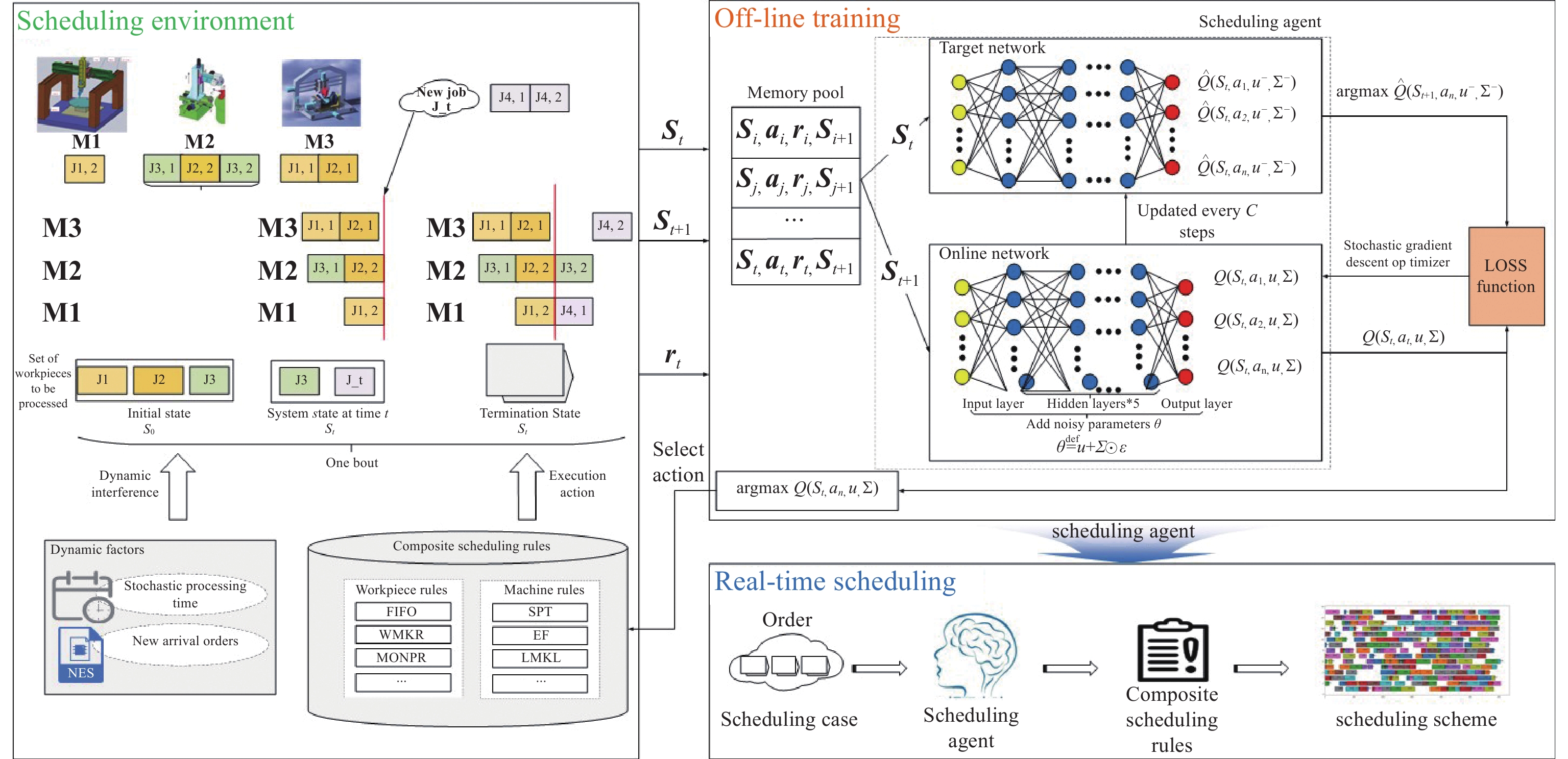
Figure 2. N-DDQN framework solving large-scale flexible job shop dynamic scheduling problem.
Here,  represents the state of the decision moment point;
  represents the instantaneous reward for moving from the previous state to the current state; A represents the set of actions; S represents the set of states; and R represents the reward function. Once the action is performed, the environment state changes to another environment state s
  , and a bonus
  is obtained. u and
  are the online network parameters.
  and
and  denote the target network parameters.
  represents a zero uniform noise vector, and
  represents multiplication by element.
1) Scheduling environment. It is an abstraction of the shop environment, which requires the initial set of artifacts  . The inserted artifact set
  is distributed on
  machine tools in the workshop according to the process route of the workpieces. The working hour of each process is not determined but follows the normal distribution. When all the machine tools in the scheduling environment are in idle states, the scheduling agent chooses the appropriate compound scheduling rules to arrange the workpiece processing by the state characteristics of the scheduling environment at the starting moment point. After that, the scheduling environment moves on to the next state when the machine tool completes a task or a fresh workpiece is delivered. After all of the workpieces that need to be processed are scheduled, the scheduling environment achieves a terminated state.
2) Off-line training. In the offline training process, there are two networks including the target and the online. The network input is the state feature  extracted from the scheduling environment, and the network output is the Q value of the corresponding action. To replace the traditional greedy strategy, noise parameters are introduced that can be trained together with neural network weights, forming a noise network called noisynet. According to the designed noisynet, the action corresponding to the maximum Q value is directly selected. The scheduling agent selects the workpiece and machine processing according to the action, and the workshop enters the next production state. The scheduling environment rewards the scheduling agent
  according to the state change, and the training is terminated until the optimal scheduling decision model is output.
3) Real-time scheduling. The verification and application process of the scheduling decision model is obtained by off-line training. When the actual production order comes, the trained scheduling decision model can be called to obtain a scheduling scheme stably and quickly, and the scheduling decision model can respond quickly to decide the appropriate compound scheduling rules at the moment point of the disturbance after the dynamic disturbance occurs. Although the acquisition of the scheduling decision model consumes a certain amount of time in the training process, it does not need to conduct the iterative search in the practical application of the scheduling decision model. In case of dynamic interference, our proposed method is a very effective method to solve the slow response speed problem of production lines and realize real-time optimization of large-scale dynamic scheduling.
3.2. Core Algorithm
The DQN [18] introduces a memory replay mechanism to break the correlation between data, thereby solving the problem that deep reinforcement learning cannot be trained. However, since the maximum value is used to determine the action selection and the target Q value estimation, the DQN often leads to the overestimation of the algorithm. For this reason, Hasselt et al. [19] proposed the DDQN algorithm to avoid the overestimation problem of the DQN algorithm by separating the selection action from the evaluation action. The DDQN first evaluates the action selection in the online network to select the action, and then estimates the target Q value through the target network. Nevertheless, like the DQN algorithm, the DDQN algorithm also needs to balance between exploration and utilization by using the  -greedy algorithm in the process of learning. As such, the DQN algorithm can lead to the stability of the model solution and the unsatisfactory scheduling strategy when solving the LSDSP with high model complexity and large action and state spaces.
Meire et al. [20] proposed an N-DQN algorithm to solve the problem of balancing exploration and utilization. In this algorithm, a parameterized noise is introduced based on the DQN algorithm which is able to be learned together with the weight in the network through gradient descent. Hence, the agent could decide which proportion to use for introducing the weight into the uncertainty and realizing automatic exploration.
In deep reinforcement learning, network weights often follow certain probability distribution, which describes the uncertainty of weights and can be used to estimate the uncertainty in prediction [21]. In the implementation process of the noisynet, a noise parameter is added at each step, and the uncertain disturbance is randomly obtained from the noise distribution. The variance of the disturbance can be regarded as an energy input of the input noise. These variance parameters are learned together with other parameters of the agent by using the gradient of the reinforcement learning loss function. Finally, the perturbation of network weights learned by the noisynet can be directly used to drive the exploration process. A noise network is a kind of neural networks whose weight and bias are disturbed by noise parameter functions. These parameters are adjusted by the gradient descent method. There are two main characteristics in the execution process of the noise network: 1) the noise is sampled before interacting with the environment in the no-hungry round, and 2) the noise remains unchanged in a round to ensure that the agent can take the same action when given the same state.
Referring to the method of noise parameter setting in Ref. [20], the noisynet is added into the network of the DDQN algorithm to replace the traditional  -greedy and form an N-DDQN algorithm according to the principle of the N-DQN in this paper. Since a set of learnable noise parameters is added to the network, the action of the N-DDQN algorithm interacting with the environment is the action corresponding to the maximum state-action value function output by the network. This makes the algorithm more stable than the traditional DDQN algorithm. The Q value calculation formula is shown in Equation (10).

Here,  represents the discount factor; a and S' represent the best action and its corresponding state in the next state, respectively;
  represents target network parameters; and
  represents the online network parameters.
Adding the noise parameters of Equation (11) to the DDQN, the Q value calculation formula of the noisynet-DDQN is shown in Equation (12).


3.3. Scheduling Problem Transformation
3.3.1. Design of State Feature
In the deep reinforcement learning algorithm, the reasonable design of state features directly affects the algorithm performance and follows the following principles. 1) The extracted state features should enable the scheduling agent to get feedbacks in a short time so that the scheduling agent can quickly select scheduling tasks for processing. 2) The state characteristics should be able to cover all the information of the whole scheduling environment. 3) The state characteristics should be closely related to scheduling objectives and action sets to avoid feature redundancy.
It is difficult to extract state features for LSFJSDSPs, and the sensitivity of state features to decision-making problems will affect algorithm accuracy. As shown in Table 2, by analyzing the scheduling problem and its optimization objectives, this paper extracts 10 state features as network inputs according to the designed reward function and the feedback state features of action sets.
Table 2. Design table of state feature
| Feature | Design consideration | Description |
| f1 | Schedule completion | Job completion rate |
| f2 | The standard deviation of job completion | |
| f3 | Reward function | Average machine utilization |
| f4 | Earliest completion time | The standard deviation of average machine utilization |
| f5 | Action set | Normalization of maximum remaining hours |
| f6 | The maximum number of remaining processes is normalized | |
| f7 | Minimum machine load normalization | |
| f8 | Normalization of minimum processing time | |
| f9 | The minimum completion time of available machine tools is normalized | |
| f10 | Normalization of the earliest arrival time of the workpiece |
3.3.2. Design of Action Set
When scheduling rules are used as the action space of deep reinforcement learning, the performance of scheduling rules directly affects the performance of deep reinforcement learning algorithms. Considering that the LSFJSDSP has two sub-actions: machine selection and job selection, the composite scheduling rules of both are designed as the action set in this paper. Panwalkar et al. [22] summarized 113 different scheduling rules. In this paper, the first-come, first-processing (FIFO) rule is selected as a work-piece selection rule to avoid too long waiting time according to the dynamic factor of the arrival of new workpieces in LSFJSDSPs. Then, with the minimum completion time as the optimization objective, two workpiece selection rules (WMKR, MONPR) and three kinds of machine selection rules (SPT, EF, LMKL) with high sensitivity to completion time are selected. Finally, three kinds of the workpiece and machine selection rules are arranged and combined to get the design table of action sets, as shown in Table 3. The nine composite scheduling rules are shown as a set of actions.
Table 3. Design table of action set.
| No. | Composite scheduling rules | Description |
| 1 | WMKR + SPT(DR1) | The workpiece with the longest remaining processing time is processed preferentially and the machine with the shortest processing time is selected. |
| 2 | MONPR + SPT(DR2) | The workpiece with the most remaining process is preferentially selected and the machine with the shortest processing time is preferentially selected. |
| 3 | WMKR + EF(DR3) | The workpiece with the longest remaining processing time is processed preferentially and the earliest available machine is selected. |
| 4 | MONPR + EF(DR4) | The work with the remaining work is selected first and the earliest available machine is selected. |
| 5 | WMKR + LMKL(DR5) | The workpiece with the longest remaining processing time is processed preferentially and the machine load is selected preferentially. |
| 6 | MONPR + LMKL(DR6) | The workpieces with the most remaining processes are selected first and the machine load is selected least first. |
| 7 | FIFO + SPT(DR7) | The first arrived workpiece is selected by the first principle, and the machine with the shortest processing time is selected principle. |
| 8 | FIFO + EF(DR8) | The first arrived work is selected and the first available machine is selected. |
| 9 | FIFO + LMKL(DR9) | The first arrived work is selected by the first principle and the machine load is selected by the least first principle. |
3.3.3. Design of the Reward Function
In this dynamic scheduling problem, for the dynamic factor of random man-hours, the mean of the processing time matrix samples is calculated as the expected makespan of all jobs by Monte Carlo sampling. The scheduling agent is given a round reward value according to Equation (13) when each matrix sample is scheduled. Since the higher the utilization rate of the machine is, the earlier the completion time is, we give the scheduling agent an instant reward so to avoid sparse rewards in the execution process of training according to Equation (14). Using the design described above, the scheduling agent is given bigger rewards and punishments than the immediate rewards at the end of the round, with the reward and penalty values set at plus or minus 10, as shown in Equation (14).

Where  (t) represents average machine utilization at time t.

Here, makespan(t) denotes the completion time of the current round.
3.4. Offline Training Process
3.4.1. Monte Carlo Simulation
Considering that the processing time obeys normal distributions, the optimization objective of this paper is to minimize the expected completion time. In this paper, the Monte Carlo simulation is taken to calculate the expected completion time. The pseudocode for calculating the expected makespan by the Monte Carlo simulation is shown in Table 4.
Table 4. Pseudo-code for Monte Carlo sampling calculating the expected completion time
| Algorithm 1: Monte Carlo sampling to calculate expected makespan pseudocode |
| 1: Input: Z processing time matrices corresponding to the workpiece to be processed |
| 2 Output: The expected completion time of all the workpieces to be processed |
| 3: for z = 1 to Z do: |
| 4: Z processing time matrices are obtained |
| 5: Calculate the makespan for each processing time matrix z |
| 6: Calculate the expected makespan for Z processing time matrices |
| 7: End for |
3.4.2. Offline Training with Noisynet-DDQN Algorithm
The whole offline training process is that the scheduling agent continuously interacts with the dynamic environment with random working hours and new job arrivals. Through continuous interactions, the scheduling agent learns the optimal scheduling policy, and stores these optimal policies in the form of neural network parameters. It can be seen that in the whole real-time scheduling framework based on the N-DDQN algorithm, offline training is the most important part of the whole real-time scheduling framework, and it is the key to determine whether the whole scheduling framework can achieve real-time scheduling optimization. The pseudocode of offline training is shown in Table 5 based on the real-time scheduling framework of the N-DDQN algorithm.
Table 5. Offline training pseudo-code based on N-DDQN algorithm real-time scheduling framework
| Algorithm 2: Pseudocode for the N-DDQN algorithm |
1: Initialize D, M, Z,  , ,  , batchsize; , batchsize; |
Initialize C, textitu,  , ,  . . |
| 2: for episode = 1 to M: |
| 3: Z processing time matrices are randomly generated |
| 4: or sample=1 to Z: |
| 5: The error is initialized to 0 |
| 6: Clear the scheduling scheme and reset the scheduling scheme |
7: The state is reset to S  |
8: Each sample process is assumed to be  |
9: for t = 1 to  do: do: |
10: Sampling noise variable  |
11: Choose action at based on argnaxQ(S,a;u,  ) ) |
12: Act, observe  and and  |
13: Store (  , ,  , ,  , ,  ) in memory pool D ) in memory pool D |
14: Randomly sample (  , ,  , ,  , ,  ) from D and compute the target Q value ) from D and compute the target Q value  |
15:  . . |
16: Use the loss function (  to perform gradient descent to perform gradient descent |
17: Update the target network parameters every C step:  , ,  |
| 18: End for |
| 19: End for |
| 20: End for |
4. Experiment and Results
4.1. Example Design
As mentioned above, the large-scale flexible job-shop dynamic model established in this paper considers two dynamic factors: the new job arrival and random working hours. However, there is no standard verification data set based on this model in the existing research. According to certain design standards, this paper generates verification examples based on the workshop environment parameters as shown in Table 6. In addition, the arrival time of new jobs is controlled by random numbers. The standard deviation of the processing hours in the table is set according to Ref. [23], which could be 1, 2, or 3 for producing varying degrees of random disturbance.
Table 6. Configuration table of workshop environment parameters based on the new job arrival and stochastic processing time.
| No. | Parameter | Description | Value |
| 1 |  |
The initial number of workpieces | {50,100, 140} |
| 2 | M | The number of machines | {20,30, 50} |
| 3 |  |
The number of new artifacts reached | 50 |
| 5 |  |
Mean processing time | Unif [1, 50] |
| 6 |  |
The standard deviation of processing time | {1,2, 3} |
| 7 |  |
Processing time |  |
| 8 | / | The number of machine tools per process can be selected | Unif [5, 15] |
| 9 | / | Number of processing steps per workpiece | Unif [5, 10] |
4.2. Experimental Design
To verify the effectiveness of the proposed algorithm framework, the experiment is configured as Intel(R) Core(TM) i5-9400 CPU @ 2.90 GHz 2.90 GHz, 8 GB of RAM, Python language, and TensorFlow version 1.4. The proposed N-DDQN algorithm is compared with the traditional DDQN algorithm and the composite scheduling rules designed by the action set. Considering that the adopted N-DDQN algorithm avoids setting the exploration parameter values of the DDQN algorithm, the parameters of the N-DDQN algorithm are set as shown in Table 7. According to Ref. [24], a neural network with one input layer, four hidden layers and one output layer is constructed, where the number of nodes in the input layer is the number of the designed state features, the number of nodes in the hidden layer is 30, and the number of nodes in the output layer is the number of the action sets designed above. In addition, the parameterized noise shown in Equation (11) is introduced into the neural network to make the network realize the adaptive search function.
Table 7. Parameter table of N-DDQN algorithm
| No. | Parameter | Description | Value |
| 1 |  |
Learning rate | 0.0001 |
| 2 | D | The capacity of the memory pool | 2000 |
| 3 | batchsize | Size of sample | 64 |
| 4 | C | Update frequency of target network | 200 |
| 5 | Max_episode | Iteration times | 5000 |
| 6 | Z | Time matrix samples of sample processing | 1000 |
4.3. Results Analysis
The offline training results directly affect the final scheduling results. The effectiveness of the offline training framework is illustrated by outputting the convergence curve of the expected completion time in the offline training process, the reward, and the punishment record of the scheduling agent. In this paper, according to the workshop environment parameters in 5, a flexible production workshop with 20 machines is taken as an example to simulate certain training data for training. The effectiveness of the designed training framework is evaluated on randomly generated instances of 50 × 20, 100 × 20, 140 × 20.
From the convergence curve of the expected completion time during training (as shown in Figure 3) and the reward change graph obtained by the scheduling agent during training (as shown in Figure 4), it can be seen that the reward and punishment record graph and the convergence curve of the expected completion time show two opposite trends: 1) the makespan decreases with the increase of the number of training steps, and 2) the reward function increases with the increase of the number of training steps. However, when the reward function tends to be stable, the convergence curve of the expected makespan becomes stable, which indicates that the scheduling agent can select the appropriate scheduling rule according to the state characteristics of the decision time at each scheduling time point. Therefore, the effectiveness of the training framework, the rationality of the designed state space, the action space, and the reward function are all verified.
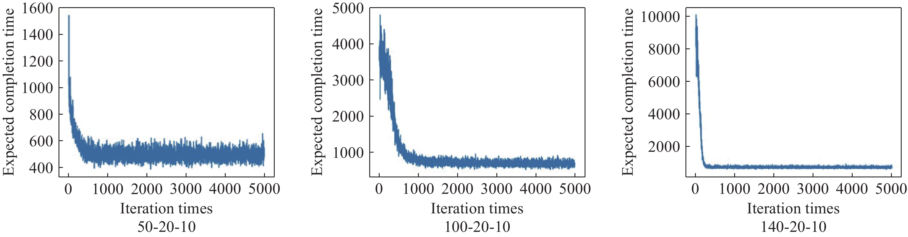
Figure 3. Iteration curve of training phase completion time.

Figure 4. Training phase scheduling agent reward and punishment record diagram.
To verify the effectiveness of the proposed real-time scheduling framework based on the N-DDQN algorithm, the obtained results are compared with the composite scheduling rules designed by the action set and the DDQN algorithm. According to Table 4, the instances are randomly generated at certain random seed. The number of initial workpieces (Nold), the number of newly arrived workpieces (Nnew), and the number of machines  all prove the generality of the algorithm. Tables 8−10 record the solution results of the six composite scheduling rules (DR1, DR2, DR3, DR4, DR7, DR8) with better performance in the action set, where the solution results of the N-DDQN algorithm shown for the time variances 1, 2, 3. The reference source is not found. The solution results of the DDQN algorithm and the real-time scheduling framework are recorded based on the N-DDQN algorithm. Table 11 records the solution results of the DDQN algorithm and the solution results of the real-time scheduling framework based on the N-DDQN algorithm.
Table 8. Comparison table of composite scheduling rules ( \begin{document}$\sigma ^{2}=1 $\end{document} )
| Example parameters | Average expected completion time of algorithms | |||||||||
| Nnew | Nold | M | N-DDQN | DR1 | DR2 | DR3 | DR4 | DR7 | DR8 | |
| 50 | 50 | 20 | 2361.45 | 3385.43 | 3353.29 | 5513.81 | 4267.82 | 3473.57 | 3186.55 | |
| 30 | 1682.06 | 2503.17 | 2464.21 | 4118.17 | 3308.43 | 2740.45 | 2420.25 | |||
| 50 | 1215.87 | 1817.48 | 1776.43 | 2934.61 | 2402.53 | 2166.88 | 1788.96 | |||
| 100 | 20 | 4162.83 | 5067.55 | 5043.19 | 7590.95 | 5714.21 | 5448.52 | 5236.54 | ||
| 30 | 2903.29 | 3771.37 | 3735.61 | 5623.99 | 4352.87 | 3890.84 | 3630.95 | |||
| 50 | 1945.47 | 2759.89 | 2721.16 | 3883.26 | 3126.84 | 3090.10 | 2752.08 | |||
| 140 | 20 | 5360.79 | 7226.84 | 7197.59 | 9593.89 | 7152.10 | 7704.74 | 7205.90 | ||
| 30 | 3644.02 | 5531.12 | 5496.52 | 7078.02 | 5429.77 | 6052.25 | 5841.68 | |||
| 50 | 2357.86 | 4196.42 | 4152.38 | 4842.63 | 3797.73 | 4996.33 | 4687.84 | |||
Table 9. Comparison table of composite scheduling rules ( \begin{document}$\sigma ^{2}=2 $\end{document} )
| Example parameters | Average expected completion time of algorithms | |||||||||
| Nnew | Nold | M | N-DDQN | DR1 | DR2 | DR3 | DR4 | DR7 | DR8 | |
| 50 | 50 | 20 | 2361.45 | 3385.43 | 3353.29 | 5513.81 | 4267.82 | 3473.57 | 3186.55 | |
| 30 | 1682.06 | 2503.17 | 2464.21 | 4118.17 | 3308.43 | 2740.45 | 2420.25 | |||
| 50 | 1215.87 | 1817.48 | 1776.43 | 2934.61 | 2402.53 | 2166.88 | 1788.96 | |||
| 100 | 20 | 4162.83 | 5067.55 | 5043.19 | 7590.95 | 5714.21 | 5448.52 | 5236.54 | ||
| 30 | 2903.29 | 3771.37 | 3735.61 | 5623.99 | 4352.87 | 3890.84 | 3630.95 | |||
| 50 | 1945.47 | 2759.89 | 2721.16 | 3883.26 | 3126.84 | 3090.10 | 2752.08 | |||
| 140 | 20 | 5360.79 | 7226.84 | 7197.59 | 9593.89 | 7152.10 | 7704.74 | 7205.90 | ||
| 30 | 3644.02 | 5531.12 | 5496.52 | 7078.02 | 5429.77 | 6052.25 | 5841.68 | |||
| 50 | 2357.86 | 4196.42 | 4152.38 | 4842.63 | 3797.73 | 4996.33 | 4687.84 | |||
Table 10. Comparison table of composite scheduling rules ( \begin{document}$\sigma ^{2}=3 $\end{document} )
| Example parameters | Average expected completion time of algorithms | ||||||||
| 50 | 50 | 20 | 2883.24 | 3886.87 | 3854.11 | 5517.40 | 4244.50 | 3883.54 | 3623.64 |
| 30 | 2171.60 | 3003.02 | 2965.50 | 4136.66 | 3332.51 | 3171.60 | 2866.95 | ||
| 50 | 1624.02 | 2317.78 | 2276.30 | 2923.58 | 2403.41 | 2624.02 | 2253.35 | ||
| 100 | 20 | 4145.50 | 5568.83 | 5539.39 | 7567.38 | 5648.95 | 5347.30 | 5604.74 | |
| 30 | 2884.88 | 4272.07 | 4238.89 | 5609.90 | 4331.00 | 4345.34 | 4069.05 | ||
| 50 | 1792.40 | 3261.43 | 3223.35 | 3878.63 | 3088.44 | 3590.82 | 2703.36 | ||
| 140 | 20 | 5345.34 | 7727.42 | 7699.73 | 9595.77 | 7122.94 | 7200.33 | 7108.55 | |
| 30 | 3655.36 | 6031.77 | 5998.54 | 7097.76 | 5448.58 | 5917.77 | 5754.51 | ||
| 50 | 2353.95 | 4697.19 | 4653.34 | 4837.53 | 3809.45 | 4995.48 | 4132.15 | ||
Table 11. Comparison table of DDQN algorithm
| Example parameters |  |
 |
 |
||||||||
| Nnew | Nold | M | N-DDQN | DDQN | N-DDQN | DDQN | N-DDQN | DDQN | |||
| 50 | 50 | 20 | 2361.45 | 2899.55 | 3072.15 | 3309.14 | 2883.24 | 3076.06 | |||
| 30 | 1682.06 | 2012.53 | 2113.08 | 2430.96 | 2171.60 | 2119.10 | |||||
| 50 | 1215.87 | 1344.67 | 1362.40 | 1748.45 | 1624.02 | 1363.92 | |||||
| 100 | 20 | 4162.83 | 4268.91 | 4144.73 | 4207.39 | 4145.50 | 4281.55 | ||||
| 30 | 2903.29 | 2990.11 | 2818.20 | 3079.04 | 2884.88 | 2827.20 | |||||
| 50 | 1945.47 | 1944.57 | 1824.56 | 2221.51 | 1792.40 | 1823.03 | |||||
| 140 | 20 | 5360.79 | 6376.08 | 5371.85 | 6409.87 | 5345.34 | 6887.19 | ||||
| 30 | 3644.02 | 4728.27 | 3640.09 | 4769.29 | 3655.36 | 5236.30 | |||||
| 50 | 2357.86 | 3398.77 | 2364.19 | 3405.82 | 2353.95 | 3843.44 | |||||
The results show that the performance of the real-time scheduling framework based on the N-DDQN algorithm is better than the performance of the composite scheduling framework. At the same time, the performance of 98% of the examples is better than that of the DDQN algorithm, and the real-time scheduling framework based on the N-DDQN algorithm has better performance as the instance scale becomes larger. The results also show that the performance of the algorithm is affected by the number of inserted jobs and machines. The more the number of machines, the smaller the expected makespan. The more jobs that are inserted, the longer the expected makespan is, and the more likely the job will not be completed within its due date.
4.4. Stability Analysis of Algorithms
To verify the stability of the real-time scheduling framework based on the N-DDQN algorithm, the variances of the processing time are set to 1, 2, and 3, respectively, according to Table 6 in order to simulate different degrees of random interference. Then, the model under offline training is saved to solve each instance under different interference. The best composite scheduling rule in the action set is the DDQN algorithm, and the real-time scheduling framework based on the N-DDQN algorithm is used to process the solution results of the three examples. The processed value is the solution deviation GAP (GAP = (C −  ) /
) /  100%), where C is the current target value, and
  is the best target value in this set of data).
According to the calculated GAP data, the box plot of Figure 5−7 is drawn, where the solid line and dashed line inside the box plot represent the median and mean of the group of data, respectively. The upper and lower edges of the rectangular box represent the upper and lower quartiles of the group of data, and the solid line outside the rectangular box represents the maximum value of the group of data. N1, N2 and N3 on the abscissa represent the variances (1, 2, 3) of processing hours that obey normal distributions. Some conclusions can be drawn as follows according to the calculated GAP data and the box plot of Figure 5−7.
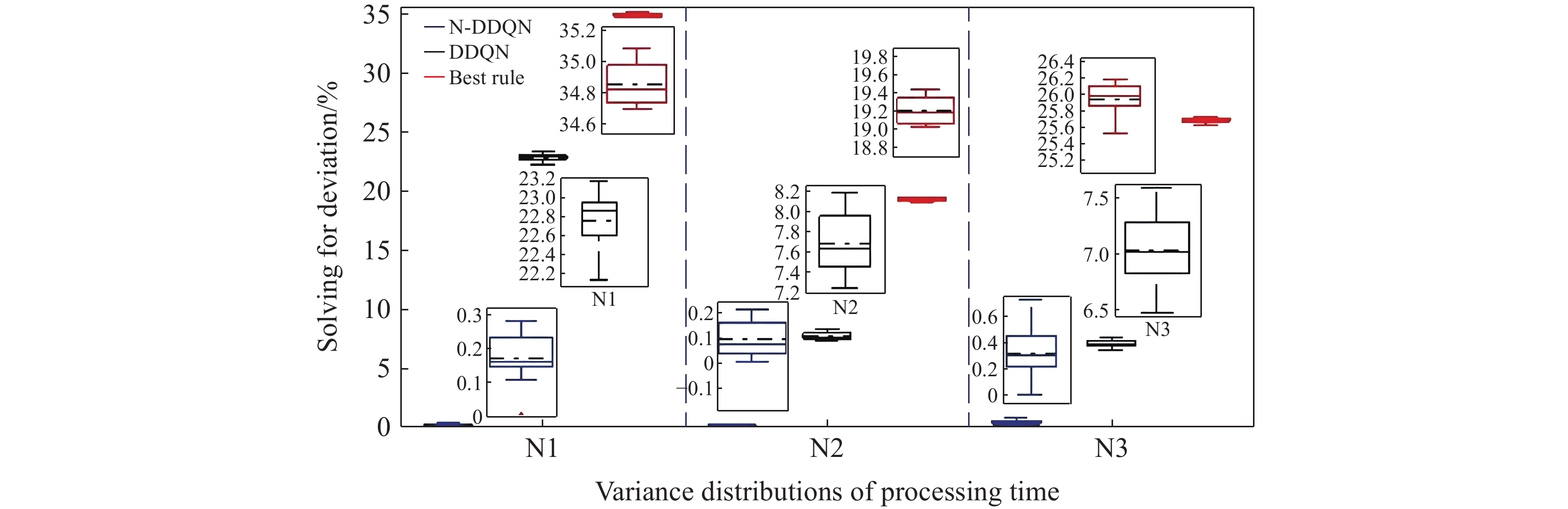
Figure 5. Results of each algorithm under different variance distributions.(50-20-50).
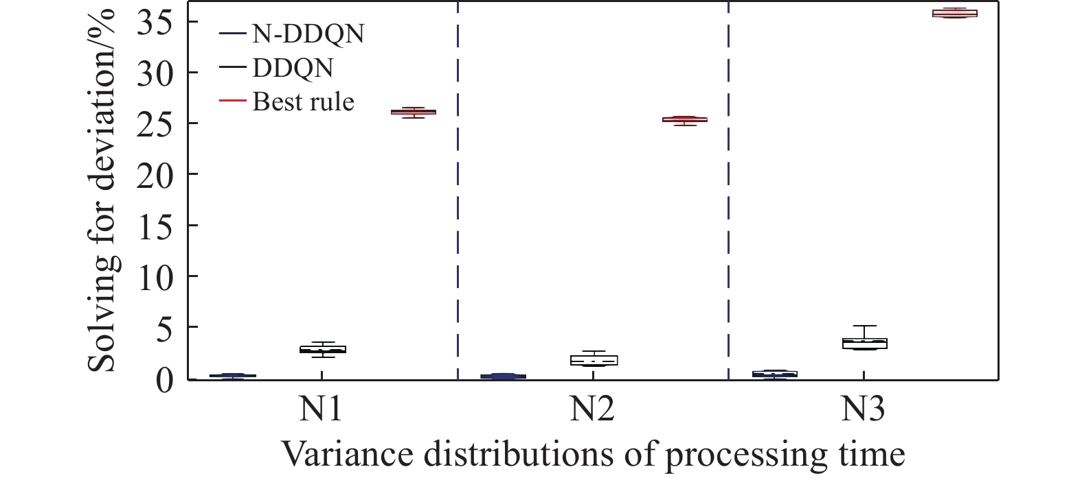
Figure 6. Results of each algorithm under different variance distributions.(100-20-50).
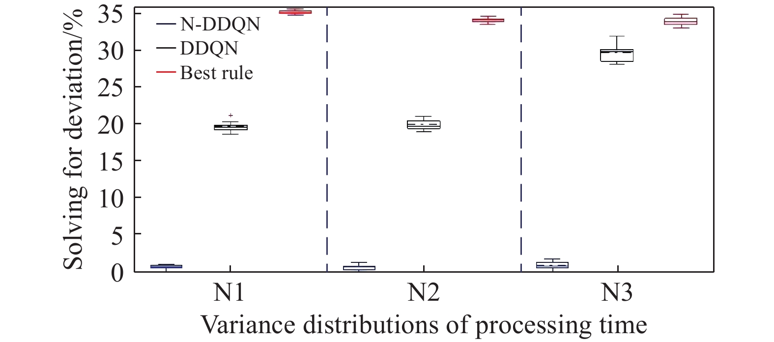
Figure 7. Results of each algorithm under different variance distributions.(140-20-50).
1) The vertical length of the rectangular box of the real-time scheduling framework based on the N-DDQN algorithm is smaller than that of the DDQN algorithm, which indicates that the results of the real-time scheduling framework based on the N-DDQN algorithm are more stable than that of the DDQN algorithm.
2) In the real-time scheduling framework based on the N-DDQN algorithm, the position of the black dotted line in the rectangular box is lower than that of the DDQN algorithm, which indicates that the deviation value of the solution data of the real-time scheduling framework is smaller based on the N-DDQN algorithm and the dispersion is lower.
3) The vertical length of the rectangular box of each algorithm becomes longer with the increase of the scale. This is because (A) the increase of the scale will lead to the expansion of the solution space; and (B) the impact of the uncertain man-hour on the scheduling results will also increase.
4) In the same scale, as the variance increases, the vertical length of the rectangular box becomes larger. The larger the variance is, the larger the interference is, and the higher the stability requirement of the algorithm is.
5) The solution accuracy of the proposed algorithm framework is higher than that of the best rule, and the solution accuracy of 50-20-50,100-20-50 and 140-20-50 instances under different variance disturbances is 36.8%, 46.1% and 54.1% higher on average, respectively.
Because the key problem of the production workshop of the enterprise is the untimely response to dynamic disturbance, it is difficult to realize real-time scheduling optimization, especially in large-scale production. Production resources are abundant and the production environment is complex and dynamic. If the dynamic disturbance is not handled in time, the production efficiency of the enterprise may be greatly affected. In LSFJSDSPs, in addition to the effectiveness and stability of the algorithm, it is necessary to verify the efficiency of the algorithm.
Table 12 records the average solution times of ten operations for the real-time scheduling framework based on the N-DDQN algorithm, the DDQN algorithm, and the six composite scheduling rules with better performance in the action set, respectively. It can be seen that the solution time of the real-time scheduling framework based on the N-DDQN algorithm is slightly higher than that of the DDQN algorithm, but only by a few seconds. This is because the addition of noise parameters increases the computational complexity of the network structure, which consumes slightly longer computing time than the DDQN algorithm. However, it can be seen from Table 11 that the solution accuracy of the real-time scheduling framework based on the N-DDQN algorithm is higher than that of the DDQN algorithm, and the solution accuracy of the three scale examples of 50-20-50,100-20-50 and 140-20-50 under different variance disturbances is 15.3%, 19.7% and 36.9% higher on average, respectively.
Table 12. Comparison table of solving time of algorithms
| Example parameters | The average solution time of each algorithm | ||||||||||
| Nnew | Nold | M | NDDQN | DR1 | DR2 | DR3 | DR4 | DR7 | DR8 | DDQN | |
| 50 | 50 | 20 | 95.21 | 47.01 | 52.34 | 46.21 | 57.83 | 49.21 | 56.24 | 87.97 | |
| 30 | 95.92 | 48.45 | 55.92 | 48.90 | 56.80 | 48.39 | 58.48 | 89.15 | |||
| 50 | 98.64 | 50.22 | 63.94 | 50.76 | 62.48 | 51.02 | 62.52 | 92.63 | |||
| 100 | 20 | 175.60 | 93.76 | 103.03 | 94.25 | 109.29 | 93.97 | 100.05 | 153.24 | ||
| 30 | 179.51 | 95.23 | 106.25 | 95.98 | 111.84 | 95.77 | 103.57 | 158.36 | |||
| 50 | 183.84 | 97.22 | 107.91 | 98.64 | 113.47 | 96.07 | 104.29 | 162.01 | |||
| 140 | 20 | 222.98 | 133.32 | 147.25 | 134.12 | 153.21 | 133.06 | 150.24 | 213.86 | ||
| 30 | 224.60 | 136.00 | 149.36 | 137.21 | 153.94 | 133.83 | 151.64 | 218.08 | |||
| 50 | 229.33 | 135.87 | 154.04 | 136.95 | 155.87 | 135.85 | 154.26 | 220.00 | |||
5. Conclusion and Perspectives
This paper has proposed a large-scale flexible job-shop dynamic scheduling model based on the N-DDQN by considering two dynamic factors: the new job arrival and random man-hours. Compared with the traditional DDQN model, the solution accuracy of the proposed algorithm in solving LSFJSDSPs is higher than that of the DDQN algorithm. Specifically, the solution accuracy of 50-20-50,100-20-50 and 140-20-50 instances with different variances (1, 2 and 3, respectively) is, respectively, 15.3%, 19.7% and 36.9% higher on average than that of the other three size examples with different variances. The superiority of the proposed real-time scheduling framework has been verified, which is the supply of solutions to LSFJSDSPs under dynamic disturbance factors. Although the algorithm performance has been improved, the present research has not accounted for the transit time, but has focused solely on decreasing the maximum completion time. In actual production, energy consumption, production costs, machine load, and other goals are also extremely important business indicators. Therefore, the proposed method will be expanded in the subsequent study. The first extension is the LSFJS problem, and the second extension is the study of the large-scale multi-objective production scheduling problem by taking into account the transportation time.
Author Contributions: Tingjuan Zheng: writing, original draft preparation; Yongbing Zhou, Mingzhu Hu: writ-ing, review, editing and visualization; Jian Zhang: supervision and condensation and summary of innovative points. All authors have read and agreed to the published version of the manuscript.
Funding: This research was funded by Major Science and Technology Project of Sichuan Province of China under grant No. 2022ZDZX0002.
Data Availability Statement: The Flexible job shop scheduling standard test set can be downloaded from: http://people.idsia.ch/~monaldo/fjsp.html.
Conflicts of Interest: The authors declare no conflict of interest. The funders had no role in the design of the study; in the collection, analyses, or interpretation of data; in the writing of the manuscript; or in the decision to publish the results.
References
- Lu, C.; Li, X.Y.; Gao, L.; et al. An effective multi-objective discrete virus optimization algorithm for flexible job-shop scheduling problem with controllable processing times. Comput. Ind. Eng., 2017, 104: 156−174. doi: 10.1016/j.cie.2016.12.020
- Caldeira, R.H.; Gnanavelbabu, A.; Vaidyanathan, T. An effective backtracking search algorithm for multi-objective flexible job shop scheduling considering new job arrivals and energy consumption. Comput. Ind. Eng., 2020, 149: 106863. doi: 10.1016/j.cie.2020.106863
- Gao, K.Z.; Suganthan, P.N.; Tasgetiren, M.F.; et al. Effective ensembles of heuristics for scheduling flexible job shop problem with new job insertion. Comput. Ind. Eng., 2015, 90: 107−117. doi: 10.1016/j.cie.2015.09.005
- Long, X.J.; Zhang, J.T.; Zhou, K.; et al. Dynamic self-learning artificial bee colony optimization algorithm for flexible job-shop scheduling problem with job insertion. Processes, 2022, 10: 571. doi: 10.3390/pr10030571
- Gao, K.Z.; Suganthan, P.N.; Pan, Q. K; et al. An effective discrete harmony search algorithm for flexible job shop scheduling problem with fuzzy processing time. Int. J. Prod. Res., 2015, 53: 5896−5911. doi: 10.1080/00207543.2015.1020174
- Mokhtari, H.; Dadgar, M. Scheduling optimization of a stochastic flexible job-shop system with time-varying machine failure rate. Comput. Oper. Res., 2015, 61: 31−45. doi: 10.1016/j.cor.2015.02.014
- Yang, X.; Zeng, Z.X.; Wang, R.D.; et al. Bi-objective flexible job-shop scheduling problem considering energy consumption under stochastic processing times. PLoS One, 2016, 11: e0167427. doi: 10.1371/journal.pone.0167427
- Shen, X.N.; Han, Y.; and Fu, J. Z. Robustness measures and robust scheduling for multi-objective stochastic flexible job shop scheduling problems. Soft Comput., 2017, 21: 6531−6554. doi: 10.1007/s00500-016-2245-4
- Zhang, J.; Ding, G.F.; Zou, Y.S.; et al. Review of job shop scheduling research and its new perspectives under industry 4.0. J. Intell. Manuf., 2019, 30: 1809−1830. doi: 10.1007/s10845-017-1350-2
- Van Den Akker, J.M.; Hurkens, C.A.J.; Savelsbergh, M.W.P. Time-indexed formulations for machine scheduling problems: Column generation. INFORMS J. Comput., 2000, 12: 111−124. doi: 10.1287/ijoc.12.2.111.11896
- Liu, M.; Hao, J.H.; Wu, C. A prediction based iterative decomposition algorithm for scheduling large-scale job shops. Math. Comput. Modell., 2008, 47: 411−421. doi: 10.1016/j.mcm.2007.03.032
- Luo, S.; Zhang, L.X.; Fan, Y. S. Dynamic multi-objective scheduling for flexible job shop by deep reinforcement learning. Comput. Ind. Eng., 2021, 159: 107489. doi: 10.1016/j.cie.2021.107489
- Luo, S. Dynamic scheduling for flexible job shop with new job insertions by deep reinforcement learning. Appl. Soft Comput., 2020, 91: 106208. doi: 10.1016/j.asoc.2020.106208
- Gui, Y.; Tang, D.B.; Zhu, H.H.; et al. Dynamic scheduling for flexible job shop using a deep reinforcement learning approach. Comput. Ind. Eng., 2023, 180: 109255. doi: 10.1016/j.cie.2023.109255
- Waschneck, B.; Reichstaller, A.; Belzner, L.; et al. Optimization of global production scheduling with deep reinforcement learning. Procedia CIRP, 2018, 72: 1264−1269. doi: 10.1016/j.procir.2018.03.212
- Song, W.; Chen, X.Y.; Li, Q.Q.; et al. Flexible job-shop scheduling via graph neural network and deep reinforcement learning. IEEE Trans. Ind. Inf., 2023, 19: 1600−1610. doi: 10.1109/TⅡ.2022.3189725
- Park, I.B.; Park, J. Scalable scheduling of semiconductor packaging facilities using deep reinforcement learning. IEEE Trans. Cybern., 2023, 53: 3518−3531. doi: 10.1109/TCYB.2021.3128075
- Mnih, V.; Kavukcuoglu, K.; Silver, D.; et al. Human-level control through deep reinforcement learning. Nature, 2015, 518: 529−533. doi: 10.1038/nature14236
- Van Hasselt, H.; Guez, A.; Silver, D. Deep reinforcement learning with double Q-learning. In
Proceedings of the 30th AAAI Conference on Artificial Intelligence ,Phoenix ,Arizona ,USA ,12 –17 February 2016 ; AAAI Press: Phoenix, 2015; pp. 2094–2100. - Fortunato, M.; Azar, M.G.; Piot, B.;
et al . Noisy networks for exploration. InProceedings of the 6th International Conference on Learning Representations ,Vancouver ,BC ,Canada ,30 April – 3 May ,2018 ; OpenReview.net: Vancouver, 2018. - Ghoshal, B.; Tucker, A. Hyperspherical weight uncertainty in neural networks. In
Proceedings of the 19th International Symposium on Intelligent Data Analysis XIX ,Porto ,Portugal ,26 – 28 April 2021 ; Springer: Porto, 2021; pp. 3–11. - Durasević, M.; Jakobović, D. A survey of dispatching rules for the dynamic unrelated machines environment. Expert Syst. Appl., 2018, 113: 555−569. doi: 10.1016/j.eswa.2018.06.053
- Han, B.A.; Yang, J. J. Research on adaptive job shop scheduling problems based on dueling double DQN. IEEE Access, 2020, 8: 186474−186495. doi: 10.1109/ACCESS.2020.3029868
- Pandey, M. How to decide the number of hidden layers and nodes in a hidden layer? 2023.