Downloads

Geng, H., Mousavi, A., Markatos, N. G., Chen, K., & Gou, X. Reliable Cost Prediction and Control for Intelligent Manufacture: A Key Performance Indicator Perspective. International Journal of Network Dynamics and Intelligence. 2024, 3(1), 100001. doi: https://doi.org/10.53941/ijndi.2024.100001

Article

Reliable Cost Prediction and Control for Intelligent Manufacture: A Key Performance Indicator Perspective

Hang Geng 1,*, Alireza Mousavi 2, Nikolaos Grigorios Markatos 2, Kai Chen 1, and Xuan Gou 1

1 School of Automation Engineering, University of Electronic Science and Technology of China, Chengdu 611731, China

2 Department of Computer Science, Brunel University London, Uxbridge, Middlesex, UB8 3PH, United Kingdom

* Correspondence: Hang.Geng@uestc.edu.cn


Received: 10 July 2023

Accepted: 11 October 2023

Published: 26 March 2024


Abstract: 
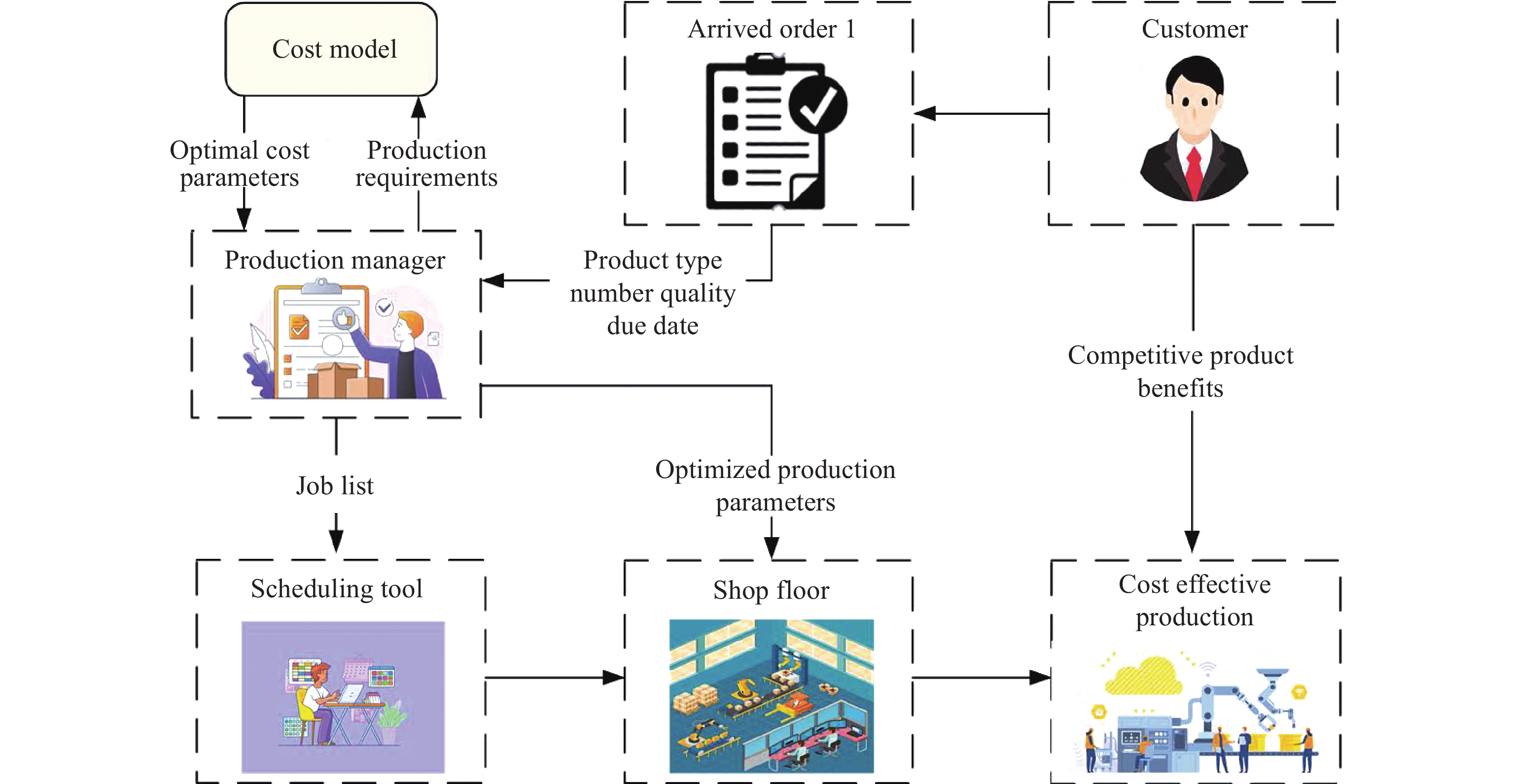
Intelligent manufacturing is facing significant challenges in adapting to the ever-changing equipment, instrumentation, process and economics. Such a trend together with the pressure to reliably control and contain production costs means that frequent adjusting decisions are required to adapt to incessant volatility imposed on manufacturing systems. Under this circumstance, cost-effective and quality-guaranteed manufacturing strategies would be the most logical route to reducing production costs. In this paper, a novel dynamical cost prediction and control (CPC) model is proposed to support collective decision-making in intelligent manufacturing, where the model output is the real-time prediction of possible manufacturing costs, while the inputs are generic manufacturing key performance indicators covering inventory, product quality, production efficiency, resource utilisation and environmental impact. This proposed CPC model distinguishes itself from existing ones for its capability to translate manufacturing data (at both the physical level and operation management level) into financial metrics that contribute to forming a common language between engineering, financial and administrative departments of an enterprise. The case study about the assembly line of optoelectronic devices demonstrates that, although different enterprise departments have different priorities, our CPC model helps them to achieve certain consensus on intended production that finally creates satisfactory profitability for the company at controlled manufacturing costs.

Keywords:

Intelligent manufacture reliable control cost prediction key performance indicator

1. Introduction

Intelligent manufacturing is a highly evolving and competitive industrial field, and a prerequisite to keep this evolvement and competitiveness is to reliably control the capital and operational expenditure while significantly reduce the final production cost [1−5]. To fulfill this goal, prediction and control of manufacturing costs becomes a major concern of both stakeholders and decision-makers, and once such prediction is obtained, business decisions and operation processes could be fully evaluated and further improved [6−10]. Generally, cost prediction and control (CPC) are vital in two aspects: 1) accurate CPC assists decision-makers in meeting business objectives such as customer satisfaction, waste reduction, and profit maximization; and 2) predicted costs can be used as manufacturing metrics to dissolve often conflicting objectives such as delivery time, production flow, energy efficiency and production quality so as to achieve balanced manufacture. This gives rise to extraordinary enthusiasm in formulating various CPC approaches whose focus is the appropriate translation of management data along with operation data into certain financial cost models to support timely yet economic decision-making of a manufacturing enterprise, see e.g. references [11−14].

Basically, even in the most mature and advanced manufacturing realms (e.g. optoelectronics), it is still a significant challenge to conduct real-time and non-stop CPC due to the colossal amount of data acquisition required by the cost analysis of every element with respect to the manufacturing process [15−18]. Moreover, most CPC approaches (e.g. the well-known activity-based CPC approach) carry out data actualization via a labor-intensive, case-based and one-off way, which are inappropriate for highly evolving production plans seeking for real-time adaptation [19−21]. In this paper, we intend to fill such a gap by building a dynamical CPC model capable of adapting itself to such possible variations of production plans. This is made possible via making full use of the capabilities (owned by the industrial internet of things) with respect to real-time tracking and tracing of manufacturing states, e.g. machine and product states.

As decision-making under a complex manufacturing environment constitutes a major concern to the management department [22−24], we are also motivated to endow the established CPC model with the ability to support the decision-making process, where the key is to reach a balance between key performance parameters (KPIs), e.g. the inventory, productivity, product quality, energy efficiency and environmental impact, of the manufacturing processes [25, 26]. Once the balance is reached, we are able to boost productivity, product quality, energy efficiency, etc. and alleviate inventory and environmental impact through the reduction of manufacturing defects and wastes.

1.1. Literature Review

Manufacturing-system-oriented CPC modeling is the integration of engineering principles, scientific theories and commercial practices for predicting the cost of manufacturing processes. Such kind of cost modeling is widely witnessed in a great variety of areas such as vehicle production, mechanical engineering, semiconductor manufacture and optoelectronic manufacture, see e.g. [27−30]. Basically, CPC techniques can be divided into qualitative and quantitative methods, where the former consists of intuitive and analogical CPC approaches, while the latter contains parametric and analytical approaches. In the intuitive CPC approach, past experience and expert knowledge are systemically leveraged to build a combination of rules and decisions to form a cost function with typical examples like the decision support systems (DSS), and case-based, rule-based, expert-based and fuzzy logic-based methodologies, see [31−33] and the references therein. The analogical CPC approach builds itself on similarity analysis that compares new products with old products of known costs in order to predict the costs of new products [34−36], while the parametric CPC approach relies on the mathematical/statistical relationship between product costs and associate parameters [37−39]. A noteworthy point is that in the analytical CPC approach, all costs of the material, labor, infrastructure, etc. are required to be added up to generate the final production costs.

To be more specific, following the idea of intuitive CPC, a knowledge-based intelligent cost model has been built in [30] to estimate the manufacturing cost at the conceptual design stage, where both material cost and operation costs (of machines) have been considered. Using the analogical CPC approach, a novel cost model has been given in [40] to estimate the operational machining costs of the microelectronic discharge. However, in such a model, the variation of workpiece/electrode parameters would lead to the change of machining time, limiting its wide applications to broader industrial scenarios. Unlike the analogical CPC approach, the parametric CPC approach requires past/historical data, and is more suitable to be applied to the early design stage without any prior knowledge about manufacturing plans [41]. As one of the most famous analytical CPC approaches, the activity-based costing (ABC) methodology has been developed in [42] to address the increasing share problem caused by the indirect fixed costs (which have significant roles in cost models of manufactured products). Note that the ABC method is, in fact, a costing model that assigns resources/costs (demanded by each production activity) to all services and products at every stage of production, delivery and marketing. Consequently, the aim of ABC is to measure and price out all activity resources together with services for customers. Unfortunately, although the ABC method is of high CPC accuracy, it can only be implemented after the completion of production, which unavoidably fails to satisfy the demand of real-time manufacture. For the latest CPC development, interested readers are referred to [43−46].

1.2. Statement of Contributions

In this article, we consider the problem of real-time CPC in intelligent manufacture which is a challenging problem that has been rarely investigated in the literature. The aim is to translate manufacturing KPIs into a universal and singular metric. We focus on a general CPC problem that features a systematic yet easy-to-deploy cost framework and addresses shortcomings of traditional detail-oriented CPC methods. Our study leads to the following contributions. 1) A novel CPC is established that translates sustainability initiatives and production strategies into real financial costs, therefore enabling operation managers/engineers to communicate with high-level decision-makers about the production process. 2) An elaborate selection strategy is designed for a series of KPIs that represent the manufacturing performance with the help of industrial partners (from the optoelectronics field) and subsequently, such KPIs are adopted as the inputs to the established CPC model. 3) A model validation process is conducted (at plants of our partners) that verifies at the shop floor, and production costs can be instantaneously reduced by tactical optimization, giving rise to high sustainability; and at the management level, proper determination of manufacturing parameters dramatically reduces the product defects, material wastes, time consumption, gas emission and energy overhead.

1.3. Organization

The remainder of this article is organized as follows. In Section 2, the CPC problem of intelligent manufacture is formulated. In Section 3, the KPI-based solution is elegantly explored with its contribution to the final production cost clearly elaborated. In Section 4, the case study on a laser device company is fully carried out whose final production cost is predicted using the proposed CPC model, where a detailed comparison is provided between the predicted cost and the real cost (data given by the financial department of the partner company) to demonstrate the applicability of the proposed CPC model. Section 5 supplies a few concluding remarks on the proposed CPC modeling method.

2. CPC Problem Formulation

In manufacturing operations, KPIs can be defined as a group of metrics that demonstrate how efficiently a company achieves its operational performance [47, 48]. KPIs are sometimes referred to as values which can be compared with internal or external targets to give certain indications of the operational performance. Hundreds of KPIs are frequently used in manufacturing industries ranging from the automobile industry to the construction industry. For instance, the emission, waste and resource utilisation (RU) in automotive fields; the quality, delivery, cost and flexibility in financial fields; the suppliers and employees in social fields; and the construction time and speed, time variation, quality, functionality, unit cost and user satisfaction in construction fields [49−51]. To sum up, each type of industry has its own indicators depending on the final business objectives.

Quality and productivity, as the crucial factors of manufacturing sustainability, are always contradicted with each other [52, 53]. The current CPC methodologies aim to mitigate this conflict by providing a cost model allowing manufacturers to appropriately opt manufacturing parameters so as to maintain the productivity at certain acceptable level, meanwhile capable of implementing zero-defect manufacture. Here, we aim to build a novel dynamical cost model to support collective decision-making in intelligent manufacturing, where the model output is the real-time prediction of possible manufacturing costs, while the inputs are five generic manufacturing KPIs.

Normally, the number of KPIs with respect to certain manufacturing environment is dependent on the business size, complexity as well as enterprise principles and priorities [54]. As suggested by our case study partner, we choose five KPIs (i.e. inventory, product quality, production efficiency, RU and environmental impact) as our focused parameters to demonstrate how effectively and efficiently the company operates. As a matter of fact, the function of the cost model is to translate the gain of each KPI into certain financial cost (i.e. the monetary value). In other words, given the desired quality and quantity of the order, the formulated model is able to output the final production cost.

Figure 1 illustrates the prediction flowchart of how such a cost model can be used to build a bridge between the newly arrived customer order and the resultant production cost. To be specific, when a new customer order arrives at the manufacturing factory, the production planner employs an underlying cost model to identify the most suitable KPIs as well as the related manufacturing parameters (about this specific customer order) that are capable of providing both low defect rate and high productivity of the overall manufacturing process.

Figure 1. Cost prediction flowchart.

Notice that it is not a one-shot process to calculate the final product cost as the calculation consists of several steps associated with several computation formulas about elaborately selected KPIs. Inspired by [28], the CPC model proposed in this paper can be established as follows:

where  is the final production cost;  is the operational cost which includes salaries of operators, machines utilization fees, maintenance and depreciation fees, set up fees and energy consumption fees;  represents the raw material cost;  defines the inventory cost; and  denotes the environmental impact cost. The four cost terms are analysed/calculated according to the previously selected five KPIs and subsequently, summed up to generate the final production cost.

In what follows, let us study how each KPI contributes to the above four cost terms as well as the final production cost.

3. KPI-Based Solution

In this section, we will explore the relationships between the aforementioned four cost terms, the five KPIs (i.e. inventory, product quality, production efficiency, RU and environmental impact) and a series of manufacturing parameters in order to determine  and . With these four cost terms in hand, we will be able to acquire the output of model (1) which is the most important factor to both customer and production manager.

3.1. Product Quality Contribution

Product quality serves as a key factor in the manufacturing process, and exerts direct influence on the final production cost. Moreover, product quality could also affect customer-manufacturer relationships such as the amount of orders, the evaluation of products, and the loyalty to manufacturers. Basically, there are numerous factors affecting product quality. For example, in cases of equipment faults, machine breakdowns and unqualified products, production managers and engineers have to stop the production process to carry out certain maintenance, called the routine maintenance frequency (RMF), in order to guarantee product quality. Basically, a low (high) RMF often indicates few (many) equipment/machine breakdowns and therefore, good (bad) production quality. More specifically, in the production of laser devices, the quality of the laser device deteriorates as the RMF of the assembly machines is out of certain range. As such, a trade-off between the product quality and RMF must be reached according to each separate order and specification that are set by customers.

Define the RMF (expressed in numbers) by  and the non-defective percentage of the produced devices by . Then, the relation between  and  is characterized by the following quadratic relationship:

where  and  are case-based coefficients to be determined. In addition, we categorize defective products into repairable and non-repairable ones as follows:

where  denotes the percentage of reparable products; and  and  represent the repairable and non-repairable percentages of the defective products, respectively.

3.2. Productivity Contribution

The proposed CPC model in (1) is a function of the RU with respect to the machine/equipment, and the RU (denoted by ) is a main measurable indicator of productivity. Generally, the RMF  is the average opening/shutting frequency (required for machine/equipment maintenance per week), and the shift frequency  (expressed in numbers) is the total opening/shutting frequency required for completing the assigned production workload per week. In this case, the RU can be formulated as follows:

Without loss of generality, the cost of machine operation  is assumed to be a quadratic function with respect to  as in many other manufacturing cases, see [55, 56] and the references therein. Note that  combines together the salaries of operators, machines utilization fees, maintenance and depreciation fees, set up fees and energy consumption fees. The detailed calculation formula of  is given as follows:

where  are cased-based coefficients to be determined by making use of the collected manufacturing data.

3.3. Efficiency Contribution

Production efficiency evaluates the performance level and the capability of the manufacturing system to not only create qualified products, but also achieve satisfactory operations along with financial performances. Generally, the lower efficiency a manufacturing system has, the higher cost a manufacturer pays. As such, production efficiency can serve as a primary index of manufacturing enterprises striving to satisfy highly-changing customer demands and occupy competitive market shares.

The proposed CPC model characterizes the KPI efficiency in terms of the raw material cost  and the operational cost . Denote  as the normal material cost and  as the normal inspection cost. Then, the calculation formulas of  and  can be established as follows:

where  is constituted by two terms, i.e. the normal material cost , and the additional material cost  required to repair defected products which are reparable; and  is constituted by four terms, i.e. the operational cost , the additional operational cost  required to repair defected products which are reparable, the normal inspection cost  required to inspect machine status, and the additional inspection cost  required to inspect machine status when repairing the defective products.

3.4. Environmental Impact Contribution

Environmental impact on manufacturing systems is becoming a major concern as most developing/developed countries are striving to reach carbon neutrality in the middle of this century. A typical approach to describing the carbon emission of manufacturing plants is the measurement of the associated energy consumption. However, due to various environmental rules/terms in different countries, environmental impact may have largely discrepant results on the final production costs. Such costs should cover the influence from qualified, reworked and unqualified production.

Denote the normal penalty for energy consumption as  and the normal penalty for used materials as . Then, the specific environmental impact onto the production cost is given as follows:

where  is the environmental cost, term  evaluates the energy consumption and penalty with respect to both qualified and unqualified products, while term  assesses the energy consumption and penalty with respect to previously defected but later reworked products.

3.5. Inventory Contribution

The inventory cost represents all overheads linked to material storage (which gradually reduces as raw materials constantly being fed to production lines) and product storage (which gradually reduces as products continuously being sold out). Although for inventory, the costs of product hold, replenishment along with replacement rely on the specific storage time, size, value and type of the stored products/materials, we here, for brevity, simply consider the inventory cost as certain fixed cost per time unit (e.g. a week).

In our industry case, this consideration is reasonable as both the raw material (e.g. the gold line, wafer fan and optical lens required by laser device production) and the product has a quite long shelf life, indicating that the inventory cost is fixed during the whole production process. Denote  as the inventory cost per week,  as the order shipping week,  as the order finish week, and  as the order starting week. Then, the detailed calculation formula of the inventory cost  is given as follows:

Up till now, we have elaborated the contributions from each KPI to the final production cost in order to determine the cost terms of the established CPC model (1). Table 1 lists the detailed computation procedure of the CPC model.

Table 1. Calculation procedure of the proposed CPC model

Step 1: Calculate the non-defective percentage of the produced device by (2).
Step 2: Calculate repairable and non-repairable percentages of defected products by (3)–(4).
Step 3: Calculate the RU by (5).
Step 4: Calculate the cost of machine operation by (6).
Step 5: Calculate the raw material cost by (7).
Step 6: Calculate the operational cost by (8).
Step 7: Calculate the environmental cost by (9).
Step 8: Calculate the inventory cost by (10).
Step 9: Sum up all KPI-based costs to determine the final production cost by (1).


4. Manufacturing Case

The modeling accuracy of the developed CPC model is verified by one real-world manufacturing scenario from optoelectronic manufacture, i.e. laser module production. In this manufacturing scenario, the RMF is selected as a controlling parameter accounting for the fact that, the RMF affects both product quality and order completion time (due date) required by customer satisfaction. It is worthwhile mentioning that the CPC model proposed in this article is artificially built to be simple in order to avoid requiring too much information from manufacturers, thereby easily adapting to a wide variety of industrial applications.

4.1. Case Study and Result

The manufacturing of laser modules is a complex and highly precise process that deals with microscale components, and any deviation is costly from the planned process and desired product quality. In the laser module assembly process, routine maintenance of the assembly machine is always required to guarantee zero-defected modules, and the manufacturing stage consists of a fast axis collimator (FAC), a slow axis collimator (SAC), and mirror and fibre lens assembly. Defects often occur when a low RMF is deployed, whereas a high RMF gives rise to excessive manufacturing costs. In the former case, the product is discarded costing on average 350-620 Euros per laser module, and in the latter case, the product is reserved yielding several hours’ production delay per day.

The proposed CPC model is tested to identify the optimum RMF via several different products and scenarios. Three different laser modules (S1-Series, D-Series and S2-Series) are used for the empirical study as well as the cost modelling of the concerned laser module assembly process. To be more specific, both S1-Series and S2-Series have 10 emitters on each laser module and share the same process flow, while the D-Series has 20 emitters on each laser module.

Figure 2 presents the relationship between the RMF and product quality rate (QR), and Figures 3 and 4 sketch the relationship between the cost of machine operation  and RU, where values of involved parameters are supplied by engineers and managers from our partner company for each specific manufacturing stage. More specifically, Figure 2 shows the ratio between the product quality versus RMF. The relationships between the cost of machine operation  and RU are illustrated in Figures 3 and 4, respectively, by the quadratic equation  for S1-Series and S2-Series, and the quadratic equation  for D-Series, where  denotes RU, and  denotes the cost of machine operation. It is observed from the production line that, as the RMF increases, the product quality also climbs.

Figure 2. Quality rate (QR) vs routine maintenance frequency (RMF) (times/week).

Figure 3. The cost of machine operation vs resource utilisation (RU) (S1-Series and S2-Series).

Figure 4. The cost of machine operation vs resource utilisation (RU) (D-Series).

For S1-Series, S2-Series and D-Series products, Figure 5 depicts the relationships between the RMF and final product cost. Referring to these figures, it is witnessed that quality control scenarios of all three products demonstrate the similar pattern of cost trends along which the final product cost reaches the minimum value. On one hand, for all RMFs, D-Series has the largest product cost, while S1-Series has the smallest product cost. On the other hand, all product costs decrease as the RMF climbs up before certain point (RMF = 12.5 times/week), and all product quality descends as the RMF continues to increase after the optimal point (RMF = 12.5 times/week). As a result, the optimal RMF with respect to the final product quality locates between 12 times/week and 13 times/week.

Figure 5. Final product cost vs routine maintenance frequency (RMF) for different products.

The relationship between the RMF and defect cost is described in Figure 6 where the defect cost is the summed cost of all defected modules. We can also observe from the figure that the quality control scenarios of all three products demonstrate similar patterns of cost trends, where all defect costs reach the minimum value with the optimum point located at the RMF of 18 times/week. In addition, the curve of D-Series starts from a higher point than that of S1-Series and S2-Series, despite the fact that all defect costs converge to the same point finally. This is because that, for a single module, the number of emitters has more significant impact on the defect cost. Additionally, one notes that the minimum defect cost is guaranteed as follows at each product scenario: for S1-Series, when the RMF is 18 times/week, the minimum defect cost is 6 Euros; for D-Series, when the RMF is 18 times/week, the minimum defect cost is 9 Euros; and for S2-Series, when the RMF is 18 times/week, the minimum defect cost is 11 Euros. As such, the minimum cost follows an expected trend which is aligned with the quality curves.

Figure 6. Defect cost vs routine maintenance frequency (RMF) for different products.

Finally, Figure 7 plots the relationship between the RMF and the final production cost (the sum of the production cost, material cost, maintenance cost etc.) of three laser modules. It can be easily seen from this figure that all relationship curves have the variation trends similar to that in Figure 5, which unveils the fact that the final product cost has a significant contribution to the final production cost. Besides, one plainly observes that products S1-Series and S2-Series have very similar production costs at any RMF, while the product D-Series has much higher production costs than that of both S1-Series and S2-Series. This coincides with the fact that S1-Series and S2-Series are similar laser modules, while D-Series is a much more advanced laser module.

Figure 7. Final production cost vs routine maintenance frequency (RMF) for different products.

4.2. Result Validation Using Expert Knowledge

According to the availability/accessibility of manufacturing data and information, two validation methods are conducted to test the designed CPC model, i.e. the direct observation and the discrete event simulation methods. As the real financial performance from our case study partner is extracted, this validation is dependent on directly comparing the financial performances of the partner company with that of the CPC model projection. When the real financial performance is unavailable, a discrete event simulation of the manufacturing process is developed in Rockwell's Arena simulation 2018 package, which adopts various random pools to predict competition time and overall annual costs.

4.2.1. Validation Approach 1: Direct Observation

The shopfloor data along with a direct measurement of product costs is taken from the shopfloor, and compared with the output of the CPC model. Table 2 lists the direct operation and management data from the accountancy department of the partner company for the same production line, the same assembly machine and the same product.

Table 2. The direct observation of operation: S1/S2/D-Series

Operation Value Range
QR 99.0 %
RU 90.0 %
Finish time 3 h per module
RMF (times/week) 12
Repairable products 0.1 %
Product selling price 650/780/1400 Euros per module


We first apply the proposed CPC model to find the nearest QR curve fitted to this case, i.e. the RMF-quality-rate curve in Figure 2 with the RMF being 12. Since the selling prices provided by the financial department (of the partner company) are, respectively, 650 Euros per S1-Series, 780 Euros per S2-Series and 1400 Euros per D-Series, we conclude that the predicted costs have deviations of 8.0%, 0.25% and 23%, respectively, from the true prices of S1-Series and S2-Series. As a result, variations of the projected CPC model have good correlations with the actually predicted product costs. Moreover, such variations would converge as the CPC model continues to be applied to the production line of laser modules.

4.2.2. Validation Approach 2: Discrete Event Simulation

The input data used is listed in Table 2 for creating divergent scenarios, and 150 scenarios are created in total for the discrete event simulation models of S1-Series, S2-Series and D-Series. The discrete event simulation model characterizes the time required for manufacturing each of these modules in the case that the model reaches its steady state. Meanwhile, the model shows the utilization of manufacturing resources (e.g. workers, machines and materials) at each manufacturing stage. The inspection time is also demonstrated with several postproduction actions (like refurbishment, recycling and replacement of product parts) also provided.

Table 3 summarizes the average production performance, finish time and RU of 150 laser modules, and Figures 8 and 9 sketch the simulation results on the finish time (the sum of both production and maintenance time) and RU. It is seen from Figure 8 that the RMF (12 times/week) and the finish time (332.33 h/150 modules (S1-Series), 331.41 h/150 modules (S2-Series), and 631.45 h/150 modules (D-Series)) fit the RMF-finish-time curve. This verifies that at the RMF of 12 times/week, the corresponding finish times are 2.33 h/per module for S1-Series and S2-Series, and 4.83 h/per module for D-Series, where the deviations are 11.44% for S1-Series, 6.15% for S2-Series and 10.52% for D-Series. Casting an eye on Figure 9, it is found that the predicted RU values (with the same RMF) are 0.9981, 0.9487 and 0.9879 for S1-Series, S2-Series and D-Series, respectively. In comparison with the relationship in Figure 2, there exist deviations of 18.13%, 8,040% and 8.2630% with respect to the RU values of S1-Series, S2-Series and D-Series, respectively.

Table 3. Simulation inputs and constraints for the use case

Parameter Value Range
QR see Figure 2
Mean RU see Figure 3
Shift time 8.0 h
Mean finish time per module 2 h
Machine setup time 0.5 h
Repairability 10%
Electrical cost 0.12 Euros per kW h
Inventory cost 67.0 Euros per day
Machine running cost per hour see Figure 3
Raw materials cost/ S1-, S2- and D-Series 350/530/620 Euros per module


Figure 8. Discrete event simulation: finish time/per week (150 modules) of S1/S2/D-Series.

Figure 9. Discrete event simulation: resource utilisation (RU)/per week (150 modules) of S1/S2/D-Series.

5. Conclusion

The challenge of transferring operation data to financial metrics has long haunted the production and financial departments in intelligent manufacture. To overcome such a challenge, a KPI based CPC model has been designed in this article that features an explicit relationship between manufacturing parameters and production costs. To be more specific, the designed CPC model is capable of translating system KPIs (with respect to interested production processes) into financial cost functions, meanwhile taking into account miscellaneous production plans, conditions and strategies emerging throughout the manufacturing life cycle. Furthermore, the CPC model has been built to be data-driven so as to precisely predict and control production costs in a reliable and real-time way, meanwhile supplying both customers and manufacturers a user-friendly, case-adaptive and decision-supportive CPC approach. Finally, real-time and historical production data (from our industrial partner in optoelectronic manufacture) has been utilized to verify the applicability of the CPC model. In the direct observation and the discrete event simulation, the first iteration of the CPC model in the shopfloor reveals that there is around 11% deviations between the average actual production cost and the predicted production cost. More inspirationally, such deviations can be gradually calibrated as the production system is gradually enriched with real-time manufacturing data. Future research directions include: 1) the establishment of CPC models for different manufacturing cases, e.g. semiconductor manufacture, robot production and 3D printing; 2) the evaluation of CPC performances based on specific user requirements, e.g. raw material selection, production lifetime and inventory periods.; and 3) the formulation of CPC models with abilities of self-calibration, self-adaptation and self-updating [57, 58].

Author Contributions: Hang Geng: original draft writing; Alireza Mousavi, Nikolaos Grigorios Markatos, Kai Chen and Xuan Gou: writing–supervision, review and editing of writing, and funding acquisition. All authors have read and agreed to the published version of the manuscript.

Funding: This work was supported in part by the Natural Science Foundation of Sichuan Province of China under Grant  23NSFSC1427,  the  National  Natural  Science  Foundation  of  China  under  Grants  U2330206,  U2230206, 62173068,  and  the  European  Union’s  Horizon  2020  Research  and  Innovation  Programme  under  Grant 820677 (IQONIC).

Data Availability Statement: Not applicable.

Conflicts of Interest: The authors declare no conflict of interest.

Acknowledgments: We would like to thank Primal Electro for providing the industrial data.

References

  1. Abu Ebayyeh, A.A.R.M.; Danishvar, S.; Mousavi, A. An improved capsule network (WaferCaps) for wafer bin map classification based on DCGAN data upsampling. IEEE Trans. Semicond. Manuf., 2022, 35: 50−59. doi: 10.1109/TSM.2021.3134625
  2. Adebanjo, D.; Teh, P.L.; Ahmed, P.K. The impact of external pressure and sustainable management practices on manufacturing performance and environmental outcomes. Int. J. Oper. Prod. Manage., 2016, 36: 995−1013. doi: 10.1108/IJOPM-11-2014-0543
  3. Almeida, A.; Cunha, J. The implementation of an activity-based costing (ABC) system in a manufacturing company. Procedia Manuf., 2017, 13: 932−939. doi: 10.1016/j.promfg.2017.09.162
  4. Amrina, E.; Vilsi, A.L. Key performance indicators for sustainable manufacturing evaluation in cement industry. Procedia CIRP, 2015, 26: 19−23. doi: 10.1016/j.procir.2014.07.173
  5. Caballero-Águila, R.; Linares-Pérez, J. Distributed fusion filtering for uncertain systems with coupled noises, random delays and packet loss prediction compensation. Int. J. Syst. Sci., 2023, 54: 371−390. doi: 10.1080/00207721.2022.2122905
  6. Cao, Q.D.; Yu, H.; Charisse, P.; et al. Is high-fidelity important for human-like virtual avatars in human computer interactions?. Int. J. Netw. Dyn. Intell., 2023, 2: 15−23. doi: 10.53941/ijndi0201008
  7. Chen, H.W.; Chang, N.B. A comparative analysis of methods to represent uncertainty in estimating the cost of constructing wastewater treatment plants. J. Environ. Manage., 2002, 65: 383−409. doi: 10.1016/S0301-4797(01)90563-8
  8. Cui, Y.; Liu, Y.R.; Zhang, W.B.; et al. Sampled-based consensus for nonlinear multiagent systems with deception attacks: The decoupled method. IEEE Trans. Syst. Man Cybern. Syst., 2021, 51: 561−573. doi: 10.1109/TSMC.2018.2876497
  9. Danishvar, M.; Mousavi, A.; Broomhead, P. EventiC: A real-time unbiased event-based learning technique for complex systems. IEEE Trans. Syst. Man Cybern. Syst., 2020, 50: 1649−1662. doi: 10.1109/TSMC.2017.2775666
  10. Dong, S.L.; Liu, M.Q.; Wu, Z.G. A survey on hidden Markov jump systems: Asynchronous control and filtering. Int. J. Syst. Sci., 2023, 54: 1360−1376. doi: 10.1080/00207721.2023.2171710
  11. Fang, J.Z.; Liu, W.B.; Chen, L.W.; et al. A survey of algorithms, applications and trends for particle swarm optimization. Int. J. Netw. Dyn. Intell., 2023, 2: 24−50. doi: 10.53941/ijndi0201002
  12. Fazli, E.; Rakhtala, S.M.; Mirrashid, N.; et al. Real-time implementation of a super twisting control algorithm for an upper limb wearable robot. Mechatronics, 2022, 84: 102808. doi: 10.1016/j.mechatronics.2022.102808
  13. Gao, C.; Wang, Z.D.; Hu, J.; et al. Consensus-based distributed state estimation over sensor networks with encoding-decoding scheme: Accommodating bandwidth constraints. IEEE Trans. Netw. Sci. Eng., 2022, 9: 4051−4064. doi: 10.1109/TNSE.2022.3195283
  14. Geng, H.; Liang, Y.; Cheng, Y.H. Target state and Markovian jump ionospheric height bias estimation for OTHR tracking systems. IEEE Trans. Syst. Man Cybern. Syst., 2020, 50: 2599−2611. doi: 10.1109/TSMC.2018.2822819
  15. Geng, H.; Wang, Z.D.; Chen, Y.; et al. Multi-sensor filtering fusion with parametric uncertainties and measurement censoring: Monotonicity and boundedness. IEEE Trans. Signal Process., 2021, 69: 5875−5890. doi: 10.1109/TSP.2021.3118538
  16. Geng, H.; Wang, Z.D.; Hu, J.; et al. Variance-constrained filter design with sensor resolution under round-robin communication protocol: An outlier-resistant mechanism. IEEE Trans. Syst. Man Cybern. Syst., 2023, 53: 3762−3773. doi: 10.1109/TSMC.2023.3234461
  17. Geng, H.; Wang, Z.D.; Zou, L.; et al. Protocol-based Tobit Kalman filter under integral measurements and probabilistic sensor failures. IEEE Trans. Signal Process., 2021, 69: 546−559. doi: 10.1109/TSP.2020.3048245
  18. Guo, X.W.; Bi, Z.L.; Wang, J.C.; et al. Reinforcement learning for disassembly system optimization problems: A Survey. Int. J. Netw. Dyn. Intell., 2023, 2: 1−14. doi: 10.53941/ijndi0201001
  19. Han, F.; Liu, J.H.; Li, J.H.; et al. Consensus control for multi-rate multi-agent systems with fading measurements: The dynamic event-triggered case. Syst. Sci. Control Eng., 2023, 11: 2158959. doi: 10.1080/21642583.2022.2158959
  20. Han, F.; Wang, Z.D.; Dong, H.L.; et al. Distributed H∞-consensus estimation for random parameter systems over binary sensor networks: A local performance analysis method. IEEE Trans. Netw. Sci. Eng., 2023, 10: 2334−2346. doi: 10.1109/TNSE.2023.3246427
  21. Hou, Y.X.; Zhang, Y.; Lu, J.Y.; et al. Application of improved multi-strategy MPA-VMD in pipeline leakage detection. Syst. Sci. Control Eng., 2023, 11: 2177771. doi: 10.1080/21642583.2023.2177771
  22. Ioannidis, S.; Xanthopoulos, A.S.; Sarantis, I.; et al. Joint production, inventory rationing, and order admission control of a stochastic manufacturing system with setups. Oper. Res., 2021, 21: 827−855. doi: 10.1007/s12351-019-00465-5
  23. Juszczyk, M. The challenges of nonparametric cost estimation of construction works with the use of artificial intelligence tools. Procedia Eng., 2017, 196: 415−422. doi: 10.1016/j.proeng.2017.07.218
  24. Kasie, F.M.; Bright, G. Integrating fuzzy case-based reasoning, parametric and feature-based cost estimation methods for machining process. J. Modell. Manage., 2021, 16: 825−847. doi: 10.1108/JM2-05-2020-0123
  25. Lei, Y.X.; Karimi, H.R.; Chen, X.F. A novel self-supervised deep LSTM network for industrial temperature prediction in aluminum processes application. Neurocomputing, 2022, 502: 177−185. doi: 10.1016/j.neucom.2022.06.080
  26. Li, X.; Li, M.L.; Yan, P.F.; et al. Deep learning attention mechanism in medical image analysis: Basics and beyonds. Int. J. Netw. Dyn. Intell., 2023, 2: 93−116. doi: 10.53941/ijndi0201006
  27. Liang, S.; Liang, J.L.; Qiu, J.L. Finite-time input-to-state stability of discrete-time stochastic switched systems: A comparison principle-based method. Int. J. Syst. Sci., 2023, 54: 1−16. doi: 10.1080/00207721.2022.2093421
  28. Luo, X.; Wu, H.; Wang, Z.; et al. A novel approach to large-scale dynamically weighted directed network representation. IEEE Trans. Pattern Anal. Mach. Intell., 2022, 44: 9756−9773. doi: 10.1109/TPAMI.2021.3132503
  29. Luo, X.; Zhou, Y.; Liu, Z.G.; et al. Fast and accurate non-negative latent factor analysis of high-dimensional and sparse matrices in recommender systems. IEEE Trans. Knowl. Data Eng., 2023, 35: 3897−3911. doi: 10.1109/TKDE.2021.3125252
  30. Ma, G.J.; Wang, Z.D.; Liu, W.B.; et al. Estimating the state of health for lithium-ion batteries: A particle swarm optimization-assisted deep domain adaptation approach. IEEE/CAA J. Autom. Sin., 2023, 10: 1530−1543. doi: 10.1109/JAS.2023.123531
  31. Manesh, M.F.; Pellegrini, M.M.; Marzi, G.; et al. Knowledge management in the fourth industrial revolution: Mapping the literature and scoping future avenues. IEEE Trans. Eng. Manage., 2021, 68: 289−300. doi: 10.1109/tem.2019.2963489
  32. Mourtzis, D.; Doukas, M.; Psarommatis, F. A toolbox for the design, planning and operation of manufacturing networks in a mass customisation environment. J. Manuf. Syst., 2015, 36: 274−286. doi: 10.1016/j.jmsy.2014.06.004
  33. Mousavi, A.; Siervo, H.R.A. Automatic translation of plant data into management performance metrics: A case for real-time and predictive production control. Int. J. Prod. Res., 2017, 55: 4862−4877. doi: 10.1080/00207543.2016.1265682
  34. Plinere, D.; Aleksejeva, L. Production scheduling in agent-based supply chain for manufacturing efficiency improvement. Procedia Comput. Sci., 2019, 149: 36−43. doi: 10.1016/j.procs.2019.01.104
  35. Psarommatis, F.; Kiritsis, D. A hybrid Decision Support System for automating decision making in the event of defects in the era of Zero Defect Manufacturing. J. Ind. Inf. Integr., 2022, 26: 100263. doi: 10.1016/J.JII.2021.100263
  36. Psarommatis, F.; May, G.; Dreyfus, P.A.; et al. Zero defect manufacturing: State-of-the-art review, shortcomings and future directions in research. Int. J. Prod. Res., 2020, 58: 1−17. doi: 10.1080/00207543.2019.1605228
  37. Psarommatis, F.; Danishvar, M.; Mousavi, A.; et al. Cost-based decision support system: A dynamic cost estimation of key performance indicators in manufacturing. IEEE Trans. Eng. Manage. 2022 , in press.
  38. Psarommatis, F.; Prouvost, S.; May, G.; et al. Product quality improvement policies in industry 4.0: Characteristics, enabling factors, barriers, and evolution toward zero defect manufacturing. Front. Comput. Sci., 2020, 2: 26. doi: 10.3389/fcomp.2020.00026
  39. Qu, B.G.; Wang, Z.D.; Shen, B.; et al. Decentralized dynamic state estimation for multi-machine power systems with non-Gaussian noises: Outlier detection and localization. Automatica, 2023, 153: 111010. doi: 10.1016/j.automatica.2023.111010
  40. Shahi, K.; Li, Y.M. Background replacement in video conferencing. Int. J. Netw. Dyn. Intell., 2023, 2: 100004. doi: 10.53941/ijndi.2023.100004
  41. Shen, Y.X.; Wang, Z.D.; Dong, H.L.; et al. Distributed recursive state estimation for a class of multi-rate nonlinear systems over wireless sensor networks under FlexRay protocols. IEEE Trans. Netw. Sci. Eng., 2023, 10: 1551−1563. doi: 10.1109/TNSE.2022.3229889
  42. Stockton, D.J.; Khalil, R.A.; Mukhongo, L.M. Cost model development using virtual manufacturing and data mining: Part II–comparison of data mining algorithms. Int. J. Adv. Manuf. Technol., 2013, 66: 1389−1396. doi: 10.1007/s00170-012-4416-5
  43. Stončiuvienė, N.; Ūsaitė-Duonielienė, R.; Zinkevičienė, D. Integration of activity-based costing modifications and LEAN accounting into full cost calculation. Inz. Ekon.–Eng. Econ., 2020, 31: 50−60. doi: 10.5755/j01.ee.31.1.23750
  44. D’Urso, G.; Quarto, M.; Ravasio, C. A model to predict manufacturing cost for micro-EDM drilling. Int. J. Adv. Manuf. Technol., 2017, 91: 2843−2853. doi: 10.1007/s00170-016-9950-0
  45. Wang, J.W.; Zhuang, Y.; Liu, Y.S. FSS-Net: A fast search structure for 3D point clouds in deep learning. Int. J. Netw. Dyn. Intell., 2023, 2: 100005. doi: 10.53941/ijndi.2023.100005
  46. Wang, M.Y.; Wang, H.Y.; Zheng, H.R. A mini review of node centrality metrics in biological networks. Int. J. Netw. Dyn. Intell., 2022, 1: 99−110. doi: 10.53941/ijndi0101009
  47. Wang, X.L.; Sun, Y.; Ding, D.R. Adaptive dynamic programming for networked control systems under communication constraints: A survey of trends and techniques. Int. J. Netw. Dyn. Intell., 2022, 1: 85−98. doi: 10.53941/ijndi0101008
  48. Xiao, H.N.; Zhu, Q.X.; Karimi, H.R. Stability analysis of semi-Markov switching stochastic mode-dependent delay systems with unstable subsystems. Chaos Solitons Fractals, 2022, 165: 112791. doi: 10.1016/j.chaos.2022.112791
  49. Wang, Y.M.; Liu, W.B.; Wang, C.; et al. A novel multi-objective optimization approach with flexible operation planning strategy for truck scheduling. Int. J. Netw. Dyn. Intell., 2023, 2: 100002. doi: 10.53941/ijndi.2023.100002
  50. Wang, Y.A.; Shen, B.; Zou, L.; et al. A survey on recent advances in distributed filtering over sensor networks subject to communication constraints. Int. J. Netw. Dyn. Intell., 2023, 2: 100007. doi: 10.53941/ijndi0201007
  51. Yi, X.J.; Yu, H.Y.; Fang, Z.Y.; et al. Probability-guaranteed state estimation for nonlinear delayed systems under mixed attacks. Int. J. Syst. Sci., 2023, 54: 2059−2071. doi: 10.1080/00207721.2023.2216274
  52. Yu, H.C.; Wu, Z.T.; Jiang, B.P.; et al. Fault section location for distribution network based on linear integer programming. Int. J. Syst. Sci., 2023, 54: 391−404. doi: 10.1080/00207721.2022.2122906
  53. Zhang, Y.H.; Zou, L.; Liu, Y.; et al. A brief survey on nonlinear control using adaptive dynamic programming under engineering-oriented complexities. Int. J. Syst. Sci., 2023, 54: 1855−1872. doi: 10.1080/00207721.2023.2209846
  54. Zhao, Z.Y.; Wang, Z.D.; Zou, L.; et al. Zonotopic distributed fusion for nonlinear networked systems with bit rate constraint. Inf. Fusion, 2023, 90: 174−184. doi: 10.1016/j.inffus.2022.09.014
  55. Zhao, Z.Y.; Wang, Z.D.; Zou, L.; et al. Zonotopic multi-sensor fusion estimation with mixed delays under try-once-discard protocol: A set-membership framework. Inf. Fusion, 2023, 91: 681−693. doi: 10.1016/j.inffus.2022.11.012
  56. Zhu, K.Q.; Wang, Z.D.; Chen, Y.; et al. Event-triggered cost-guaranteed control for linear repetitive processes under probabilistic constraints. IEEE Trans. Autom. Control, 2023, 68: 424−431. doi: 10.1109/TAC.2022.3140384
  57. Zou, L.; Wang, Z.D.; Han, Q.L.; et al. Tracking control under round-robin scheduling: Handling impulsive transmission outliers. IEEE Trans. Cybern., 2023, 53: 2288−2300. doi: 10.1109/TCYB.2021.3115459
  58. Zou, L.; Wang, Z.D.; Shen, B.; et al. Moving horizon estimation over relay channels: Dealing with packet losses. Automatica, 2023, 155: 111079. doi: 10.1016/j.automatica.2023.111079