
Downloads
Download
Additional Files
Download - Supplementary Materials


This work is licensed under a Creative Commons Attribution 4.0 International License.
Article
Analysing the effect of a dynamic physical environment network on the travel dynamics of forcibly displaced persons in Mali
Boesjes Freek 1, Jahani Alireza 2, Ooink Bas 3, and Derek Groen 2,*
1 Utrecht University, Heidelberglaan 8, Utrecht, Utrecht 3584 CS, the Netherlands
2 Computer Science Department, Brunel University London, Wilfred Brown Building, Kingston Lane, Uxbridge UB8 3PH, UK
3 Blue Team Intelligence, Jan Aertshof 3, Hoevelaken 3871 WH, the Netherlands
* Correspondence: Derek.Groen@brunel.ac.uk
Received: 7 September 2023
Accepted: 30 January 2024
Published: 26 March 2024
Abstract: As of 2023, the world has approximately 100 million refugees, many of whom have been displaced by violent conflicts. Accurately predicting where these people may go can help non-government organisations (NGOs) and other support organisations to more effectively help these refugees. In this paper, we extend the existing flee migration forecasting model which models migration using intelligent agents with a dynamic network that represents the physical environment. In doing so, we integrate time-dependent data into four different characteristics from three public data sources. We obtain data from aspects such as the slope, drainage, soil and infrastructure, and use these aspects to systematically modify the movement preferences of forcibly displaced agents in the flee model. We showcase our approach by applying it to the 2012 northern Mali conflict. We find that numerous routes previously deemed traversable are actually inaccessible for prolonged periods according to sensor data, and a range of off-road routes are instead traversable for vehicles. We also perform a validation comparison with the original modelling approach, and find that our revised representation of travel routes leads to a reduction of 4.5% in the averaged relative difference. Our approach can be reused in other flee conflict contexts, of which five are present in the EU-funded ITFLOWS project alone. Our work provides the ability to represent a dynamic physical environment and potentially improves the simulation accuracy in a range of flee conflict situations.
1. Introduction
The climate change is likely leading to increased risk of conflicts, especially in developing countries, which results in more forcibly displaced people (FDP) [1, 2]. Understanding the movements of FDP could help policy makers and humanitarian organisations to provide better targeted sheltering and facilities [3]. In this regard, several studies have been performed on simulating refugee movements in a city or community [4−8] or even in the context of a facility location problem [9, 10]. Furthermore, several frameworks have been developed to support the creation of computational refugee models [11−13].
One of the recent approaches for migration modelling is agent-based modelling (ABM), which relies on a decentralised simulation approach to study social interactive systems and people movement [3, 5, 14]. ABM has a distinct advantage that assumptions (on the behaviour of individual people and interactions) can result in realistic complex systems at the population scale. For instance, the modelling of environment-migration linkages [15]. In addition, ABM can be used in circumstances (where there is limited or no training data) to complement machine learning approaches (e.g., [16, 17]) in regards to forecasting efficacy. Examples of ABM models in forced migration include models of events in refugee settlements (e.g. [18]), models of refugees within urban communities (e.g., [19]) as well as models of capturing the values of refugees [20, 21].
Flee [22] is an ABM that models the movement of FDP. Flee agents representing people are spawn on a graph of locations and routes, and they move along this graph from their original (conflicts) location to find a suitable destination (e.g., a refugee camp).The flee has been validated against a range of historical conflicts [3, 23], and enhanced to run efficiently using supercomputers [24, 25]. Note that flee does not resolve several important aspects. For instance, although flee supports for precipitation and river flood levels [26], it does not comprehensively incorporate the effects of the climate change and physical environment. This affects the FDP movement behaviour and the chosen destinations in many conflict settings. In addition, forecasting models for FDPs are not available and do not incorporate these effects in a systematic way.
Explicitly mapping and classifying the physical environment can be valuable as opposed to relying on route planners from open mapping software. This allows for simulating the paths that people will most likely take towards their destination, when clearly discernible roads are absent or existing roads become inaccessible. In addition, this allows us to incorporate climate and weather effects which particularly influence physical environment properties such as wet or submerged terrains, soil quality, and/or available infrastructure.
In this paper, we present a new dynamic physical environment network (DPEN) model that estimates the effort (or cost) required to move between two locations in a migration model. We incorporate data from four essential aspects of the physical environment (relief, drainage, soil and infrastructure) and model these aspects depending on seasonal weather and climate patterns. We present how this model representation affects the accessibility of routes in Mali over time, and demonstrate how this model can be used to introduce seasonal climate and weather effects in a flee-based migration forecast.
2. Methods
Our main tools consist of the DPEN model and the flee migration model, and the migration model is used to demonstrate the added value of our DPEN. We will describe our DPEN model in detail below. The flee migration model has already been presented initially [3], and the modifications have been made for version 2.0 in [19]. We also present and validate a coupled model, where the DPEN model informs the assumptions (in terms of environmental accessibility) in flee. We perform our comparison tests using flee 2.0 and compare the DPEN-informed flee model with the model using a static spatial environment.
Physical environment: Our DPEN consists of two parts: 1) a set of cost rasters for each interconnected pair of locations per season and 2) a dynamic accessibility network that uses the cost rasters to adjust the weights of routes in the flee location network over time. A change in the route weight in a flee 2.0 location graph results in a proportional increase of the travel time and a proportional decrease in the likelihood that such a route will be picked by displaced people (if alternative routes are available).
The cost raster is used to calculate the accessibility of spatial areas between two locations. It is a spatial grid that contains values of four distinct features derived from three data sources. The grid is built using the ArcGIS model builder (See Figure 1). We provide an overview of these features and their data sources in Table 1. The DPEN modelling process contains four phases: (i) classify each area in terms of the surface, drainage, slope and infrastructure (linked to the four input data types in Table 1); (ii) calculate the speed multiplier for each area; (iii) combine the areas into a raster and convert the speed multiplier to a travel time cost multiplier; and (iv) use the raster to find the cheapest route and store the cost of this route for each season in a flee input file. Full details on cost raster construction are available in ESM of Section B.
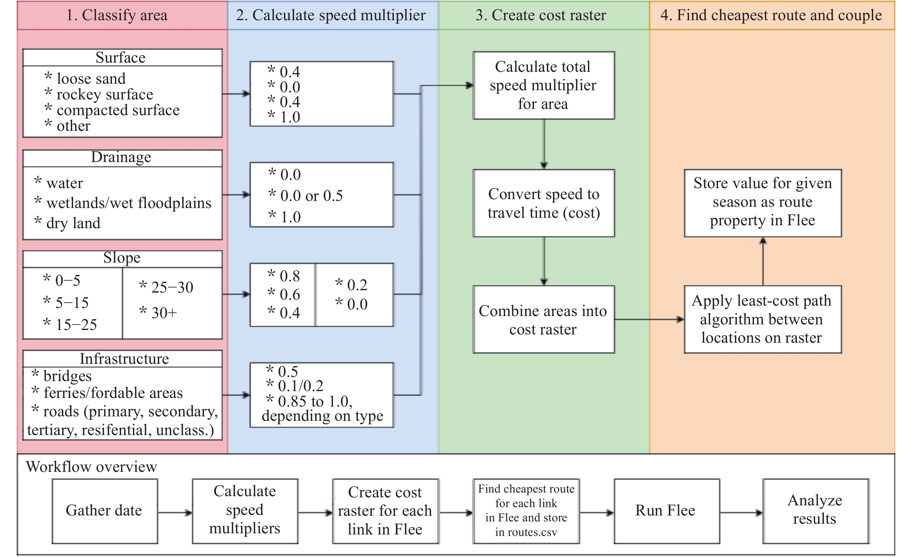
Figure 1. Architectural overview of the DPEN model, as well as the step required to create and apply the cost raster. A detailed diagram on the initial construction of our approach can be found in ESM Section B, while a detailed technical specification can be found in ESM Section D.
Table 1. Summary of data used in the study
| Type | Feature | Data | Seasonality |
| Relief | Slope – percentage of incline – non-seasonal feature | JAXA ALOS Global 30m DSM (2021) | Negligible effect |
| Drainage | Presence of open water and wetlands / floodplains – seasonal feature | Sentinel 2 – Indexed satellite images (NDMI / Wetlands in Water (WiW)) | Major effect |
| Soil | Surface material – loose sand, rocky surfaces and compacted sand/gravel/grassland– partially seasonal feature | Sentinel 2 – Esri Land Cover 2020 | Minor effect |
| Infrastructure | Presence of roads, bridges, ferries or fordable river sections –partially seasonal feature | Open Street Map; Esri Land Cover (2020) | Minor effect |
The cost rasters change over time due to seasonal weather patterns affecting the data on drainage, soil and infrastructure. In our case, we perform simulations starting in dry season 1 on February 29th 2012, continuing to wet seasons 2 (April-June) and 3 from July-September, followed by dry season 4 from October, until completion on December 25th 2012. For each season, we plot the least-cost paths through the cost rasters and use these costs to define the dynamic link weights in the DPEN.
Flee configuration: Traditionally, people are represented as autonomous and intelligent agents that move over a largely static location graph network. With the inclusion of our DPEN, we introduce dynamic (seasonal) variations in this graph. For this work, we give a modified version of flee 2.0, first presented in [19], such that it can support the results of our DPEN model and seasonal changes in the location network 1. In particular, our link weights are dynamic over time and are based on the travel time costs (derived from cost raster calculations), whereas the original link weights are static values derived from distances using the bing maps route planner (see ESM Section A for details on route definitions in flee). We use the default flee 2.0 settings [19]. We demonstrate how the DPEN affects migration forecasting using the Mali 2012 conflict setting, which has previously been used in [3]. Here, we use the DPEN model to study the effects of the physical environment on the available travel routes in Mali, where a civil war erupted in the northern part of the country [27, 28] in 2012. In general, this particular conflict has led to hundreds of thousands of displaced people [29−31].
Validation measures: In addition to the graph comparison, we also use three validation measures to quantify the validation performance of our DPEN-informed model: the root mean square error (RMSE), normalized root mean square error (NRMSE), and average relative difference (ARD). To perform the validation, we compare our model predictions in this historical setting with UNHCR data (see [3] for details).
The RMSE is commonly used to quantify the model performance [32]. It is the square root of the average squared errors between the simulated or projected values and the observed values, which allows the comparison of average errors (Equation 1).

In Equation (1),  represents the model error, or the difference between the observed and the simulated values, at iteration
  .
.  represents the total number of values [32]. We calculate the NRMSE via dividing the average RMSE values per camp by the maximum number of asylum seekers/ refugees who stay in the camp during the simulation according to UNHCR data. The result is a value between 0 and 1 for each category. The ARD, developed by the flee-team for determining the accuracy of the simulations [3], indicates the averaged relative difference between the simulated camp arrival numbers versus validation data by UNHCR. Here, the denominator Ndata,all indicates the total number of displaced people on a given day according to the validation data (normally thousands to millions of people, depending on the exact crisis situation on that day). The ARD does not square arrival differences. This follows the philosophy that in a humanitarian context, each human life should hold equal importance. We calculate the ARD across two ensembles of ten simulations, where one ensemble uses the original flee model and the other uses our DPEN-informed (or coupled) model. The ARD is calculated as follows:

The number of refugees found in camp  from the set of all camps
  at time
  is given by
  based on the simulation projections, and by
  based on the observed UNHCR data. The total number of refugees reported in the UNHCR-data is given by
  [3]. If the result is 1.0, it indicates that 50% of the simulation is wrong. An output of 0.0 means that the simulation is completely correct.
3. Results
In this section, we present our main results from two different aspects. First, we investigate the network itself, and assess to which extent the network itself is dynamic, and to which extent the generated travel times match our observations. Second, we investigate how the flee simulation performs when using our DPEN, and compare its validation performance relative to a flee simulation that features a conventional (static) location graph.
4. DPEN
To provide an overview of the dynamic nature of the DPEN, we present a comparison of the routes generated for season 1 with those generated for season 3 in Figure 2.
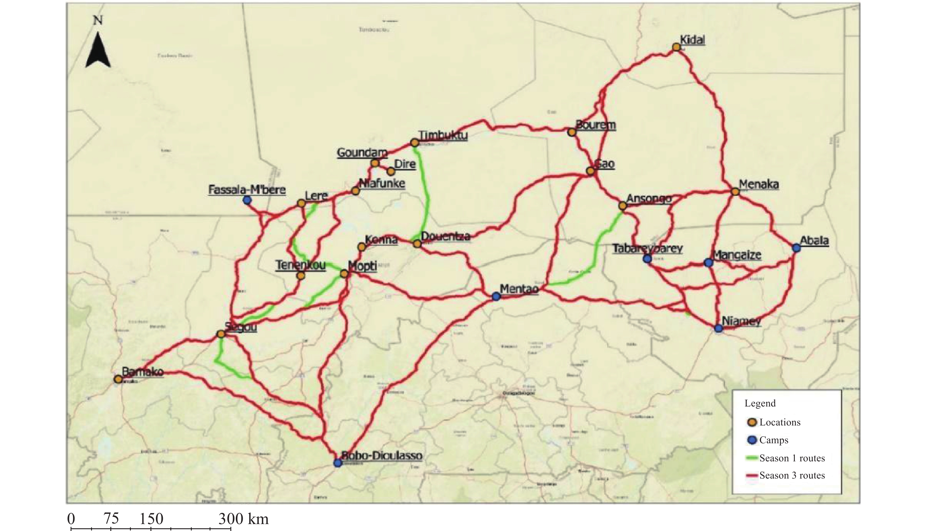
Figure 2. Overview of route accessibility differences between a dry and wet season. Routes unavailable in season 3, but available in season 1 are indicated in green while routes available in season 3 are indicated in red. In season 1, where applicable green routes between any two locations are chosen instead of red routes.
Here, the routes generally follow the major roads, unless large shortcuts are possible, or road connections or river crossings are inaccessible. Routes merge on the same path in several cases where major roads are present. For instance, the route from Ségou towards Bobo-Dioulasso includes a detour to meet-up with the highway towards this city. This is because the speed multiplier values for the roads are higher than the off-road speed multiplier values. The route distance differences sometimes amount to hundreds of kilometres and include changes in river crossing accessibility, e.g. due to the lack of fordable areas in seasons 1 and 4. We provide a full list of route changes in ESM of Section C.
We test the accuracy of travel times (and thus the weighted distance) and the plotted paths for the routes by using the Google Maps route finder. By using a route planner like Google Maps, only certain routes can be checked because off-road routes are not included in this route planner. We are able to perform verification for routes where the travel time stays roughly the same throughout the seasons and where the travel occurs via official roads. We test all routes meeting these criteria, and present our comparison results in Table 2. Here, we compare the average calculated route travel times in our DPEN with those observed using the Google Maps route planner.
Table 2. Validation comparison of averaged route travel times calculated using our cost rasters, and those estimated by the Google Maps route planner
| Start point | End point | Average simulated travel time (all seasons) | Observed travel time (Google Maps) | Absolute difference |
| [hours] | [hours] | [%] | ||
| Bamako | Segou | 3.4 | 3.5 | 2.9 |
| Bamako | Bobo-Dioulasso | 7.8 | 9.3 | 16.1 |
| Segou | Bobo-Dioulasso | 6 | 6.5 | 7.7 |
| Segou | Mopti | 4.8 | 5.5 | 12.7 |
| Mopti | Bobo-Dioulasso | 6.7 | 7.5 | 10.7 |
| Douentza | Gao | 5.7 | 7.8 | 26.5 |
The simulated routes follow roughly the same track (for each of the tests) as the route planner in Google Maps. This indicates that compared to on-road travel, the speed multipliers for off-road travel are within proportions, and the hierarchy of resistance is accurate. In other words, on-road travel is preferred if this option is available.
The tests for travel time show that on average, the difference in travel time for the routes is ~13% (see Table 2). This might not represent the actual travel time difference between simulated routes and real-world routes, because not all routes are included in the comparison. The comparison does show that the speed multiplier is roughly 87% accurate for roads in combination with the maximum speed value. Furthermore, for each of the tested routes, the simulated travel time is lower than the observed travel time. This means that the speed multiplier value and the maximum speed are more optimistic than reality. Thus, in reality, travel takes longer than simulated. We consider further inspection and calibration of these values to be the future work.
To summarise, the routes do follow the same track, which indicates an accurate ratio of speed multipliers between road and non-road values. Note that on-road travel speeds are slightly too optimistic. To more accurately represent reality, the maximum speed or the speed multipliers for roads used in the simulation should be reduced. For the off-road travel, the accuracy of the plotted routes, the multipliers and the maximum travel speed remain unknown.
5. Validation Comparison
We present the difference in the RMSE and NRMSE for each camp location in Table 3.
Table 3. Detailed RMSE and NRMSE comparison by camp. Results are averages over 10 simulation runs. The RMSE difference equals to “RMSE new” minus “RMSE original”, and is given both in an absolute value and as a percentage of the original RMSE value
| RMSE original | NRMSE original | RMSE new | NRMSE new | RMSE Difference | RMSE Diff [%] | |
| Fassala-Mbera | 14211 | 0.26 | 13215 | 0.24 | −996 | −7.01% |
| Mentao | 1268 | 0.18 | 1517 | 0.22 | 249 | 19.64% |
| Bobo-Dioulasso | 632 | 0.31 | 613 | 0.30 | −19 | −3.01% |
| Abala | 1491 | 0.13 | 1749 | 0.15 | 258 | 17.30% |
| Mangaize | 477 | 0.14 | 745 | 0.22 | 268 | 56.18% |
| Niamey | 4026 | 0.62 | 3721 | 0.57 | −305 | −7.58% |
| Tabareybarey | 2696 | 0.43 | 2640 | 0.42 | −56 | −2.08% |
| Overall | 24801 | − | 24200 | − | −601 |
In general, we find that the RMSE of our DPEN-informed model is slightly lower than that of the original model, although the results differ greatly per camp. As discussed in the visual validation comparison above, we see increases in the error particularly for three camps in Niger, Mangaize, Abala and Mentao. All three camps are relatively small. These increases could indicate that the routes in Niger (which are not covered by our DPEN) have a bias or oversimplification that has been exposed by the introduction of the more detailed DPEN model.
A second method for comparing the results is to use the Normalized Root Mean Square Error (NRMSE), which is calculated by dividing the average RMSE values per camp by the maximum number of refugees who stay in that camp during the simulation. The result is a value between 0 and 1 for each category. The NRMSE is rounded off to two decimals in Table 3. The NRMSE difference is identical to the RMSE difference, apart from the rounding difference. The NRMSE values provide a clearer picture about the validation performance of each individual camp relative to others. In particular, we find that our coupled model leads to an improved validation result for camps that perform relatively poorly with the original model. This leads to a deterioration of results for camps that perform relatively well with the original model.
Because the weights of routes change over time in our coupled model, we also calculate the NRMSE seasonally per location. All runs start on February 29th 2012 (season 1), continue into the wet seasons (season 2 from April 1st and season 3 from July 1st), followed by again the dry season (season 4 from October 1st), until completion on December 25th 2012.
For this seasonal analysis, we use the maximum number of refugees per season to normalise the seasonal data, not the maximum number for the whole run per location. This allows us to compare between seasons for the same location, as well as between locations in the same season. We present the seasonal RMSE values by the camp in Figure 3 (top) and the differences between the two models in Figure 3 (bottom). Here, the “Total” field in these figures indicates the error of predicting the total number of arrivals across all camps (not the average of the errors of the various camps).
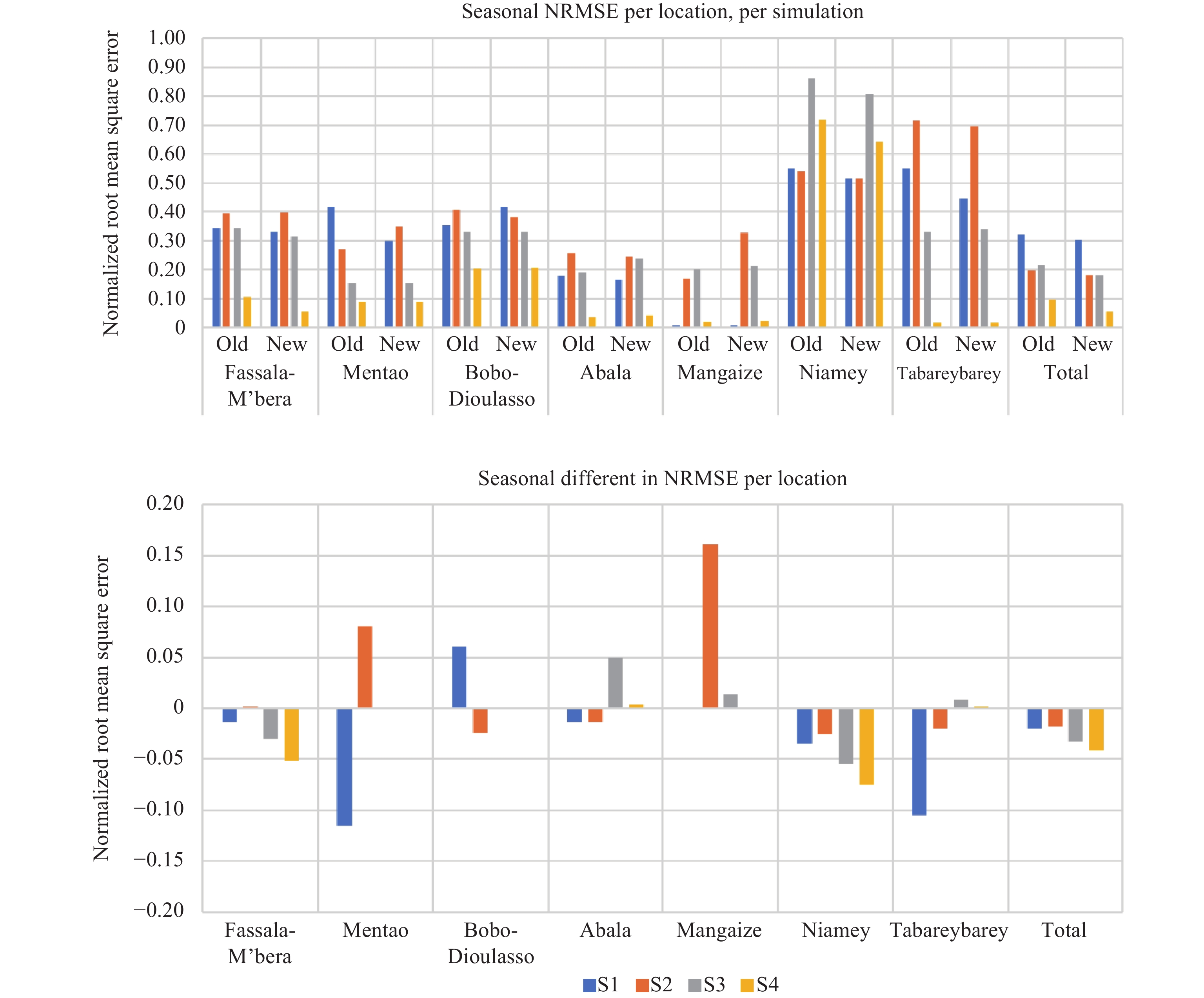
Figure 3. Top: RMSE normalized per season. Bottom: Difference in normalized RMSE scores between our simulations presented above, and Flee 2.0 simulations that do not feature a physical environment model. In both plots the error in predicting the total number of arrivals across all camps is indicated by the Total field on the right (this is not an average of the errors of the various camps) and seasons 1 to 4 are indicated using S1 to S4 symbols.
The overall NRMSE values for the four seasons are, respectively, 0.34, 0.37, 0.33 and 0.16 for the original code, and 0.31, 0.39, 0.32 and 0.14 for our new coupled model. We provide a full matrix of NRMSE values in ESM of Section E. Here, the overall NRMSE is the highest in season 2 in all cases, and the lowest in season 4. We can also recognize trends seen in earlier analysis, such as the relatively high error trends for Niamey.
To inspect these seasonal changes between the old and new runs, we present the difference in NRMSE per location per season in Figure 3 (bottom). Here, we see that the DPEN-informed model delivers a clear reduction in the error in season 1 (except for Bobo-Dioulasso) which spans the first 30 days of the forecast. We then observe an increased error for Mentao and Mangaize in season 2 (when the partial border restriction in Niger is in place), followed by negligible differences in season 3 and again the error improvement in season 4. According to Table 2, the DPEN-informed model is more stable in the near-term forecasting context, fluctuating between NRMSE of 0.3-0.35 in the first two seasons. In the original flee runs, this fluctuation is larger, between 0.42 and 0.27.
Considering the low NRMSE for season 4, in our simulations of flee, we see a somewhat lower validation error towards the end, as more camps are filled up to capacity. Capacities in the original validation setting are set according to the highest population value recorded at any point in the time period, and we chose to preserve this configuration in order to ensure a like-for-like comparison. In forecasting scenarios, where camp capacities may not be easily estimated in advance, the code is likely to deliver a higher error in such distant time periods. At the same time, this period begins only 280 days of the simulation, and is therefore likely to be of the least importance in a forecasting context.
The total ARD for the original flee runs is 0.361, while we obtain 0.345 for the DPEN-informed model, which indicates the improvement of 4.4 percent points. Note that this ARD is slightly different to that in previous publications (e.g. [3]) due to the use of the flee 2.0 ruleset, as well as an updated location graph. The improvement in ARD is somewhat higher than the RMSE improvement, primarily because the increased large error in the small Mangaize camp is not squared when using this measure.
6. Discussion
In this paper, we have presented a systematic approach to represent the physical environment in migration simulations by using a DPEN modelling approach. By combining information on four physical environment characteristics from three different data sources with the flee location graph, we are able to create effective representations of the physical environment, taking into account seasonal effects and producing travel time calculations largely consistent to those made by commonly used route planners. We have also performed a validation study to compare our improved code with the baseline flee 2.0 relying on a static routing network environment. We have found that in the majority of cases, our approach delivers a slightly reduced validation error (2 to 10% lower) when applied to the Mali 2012 conflict context.
Keeping in mind that validation data in humanitarian settings is notoriously noisy, incomplete and biased, the larger contribution of using this DPEN is that it enables the flee code to accurately represent commonly used routes which are off-road and not captured by tradition (on-road) route planners provided by e.g. Google Maps or OpenStreetMap. In addition, the use of this DPEN leads to the removal of roads that cannot be travelled during certain seasons, e.g. flooding. These two contributions do come at a price in two areas, namely, the requirement to increase the complexity of the model and invest effort to introduce the DPEN.
Constructing a dynamical network representing the physical environment is time-intensive, and several data sources need to be available to make the representation to be sufficiently accurate. Because seasonal effects are repetitive in nature, it is possible to perform such work for specific countries in advance. With advance preparations, DPENs can be used in emergency flee migration forecasts without any increase in development time during that phase (see [33] for a detailed discussion about these aspects).
Adding realistic routing to migration simulations is essential to safeguard their long-term predictive accuracy. Implementing DPENs for conflicts is labour-intensive and challenging for an academic group such as ours. Assuming that we are not bestowed with resources to do such work manually, we intend to look into methods to reduce the effort intensity of developing DPENs, and enable automated model construction in the context of flee simulation. For instance, as a feature in the FabFlee automation tool [23, 34]. Other future research directions include the definition of simplified DPEN models that can be applied more quickly in times of crisis, or less sensitive to the local availability of certain types of data. In addition, DPENs could include economic components (such as formability) to support the modelling of internally displaced people. Lastly, we identify a clear need to include more systematic estimation of camp capacities in both the validation and forecasting context. Limitations in the current estimation techniques introduce artefacts in our results in later phases, and further research is needed to develop a more realistic method for estimating camp capacities.
Supplementary Materials: Electronic Supplementary Material for this paper is available at: https://www.sciltp.com/journals/ijndi/2024/1/348/s1.
Author Contributions: Boesjes Freek: wrote the initial manuscript, implemented the algorithms, performed the background research and performed the simulation tests. Jahani Alireza: assisted in the background research, in analysing the simulation results and provided input on the humanitarian aspects. Ooink Bas: supervised Boesjes Freek during his project and provided essential technical contributions on developing the DPEN. Groen Derek: provided overall supervision and technical support on the Flee-related implementation aspects. DG also prepared the manuscript for initial journal submission and incorporated the changes needed for the revision requests.
Acknowledgments: AcknowledgmentsWe are grateful to Judith Verstegen from the University Utrecht for her supervisory support and feedback on this manuscript, and to Ron van Lammeren from Wageningen University for his supervisory support. This work was supported by the ITFLOWS project and the HiDALGO project, both of which have received funding from the European Union’s Horizon 2020 research and innovation programme under grant agreement No 882986 and 824115, respectively. In addition, this work was supported by EPSRC under grant agreement EP/W007711/1.
Funding: This work was supported by the ITFLOWS project and the HiDALGO project, both of which have received funding from the European Union’s Horizon 2020 research and innovation programme under grant agreement No 882986 and 824115, respectively. In addition, this work was supported by EPSRC under grant agreement EP/W007711/1.
Data Availability Statement: The exact code used for this work is available here: https://github.com/djgroen/flee/tree/pt-accessibility; All input files are available here: https://github.com/djgroen/FabFlee/tree/aed751fd10333ed4394578f48133b6cb0e733242/config_files/mali-freek; Output files can be generated using the code and input files (see https://flee.readthedocs.io for instructions).
Conflicts of Interest: The authors declare no conflict of interest.
Acknowledgments: We are grateful to Judith Verstegen from the University Utrecht for her supervisory support and feedback on this manuscript, and to Ron van Lammeren from Wageningen University for his supervisory support. This work was supported by the ITFLOWS project and the HiDALGO project, both of which have received funding from the European Union’s Horizon 2020 research and innovation programme under grant agreement No 882986 and 824115, respectively. In addition, this work was supported by EPSRC under grant agreement EP/W007711/1.
References
- Abel, G.J.; Brottrager, M.; Cuaresma, J.C.; et al. Climate, conflict and forced migration. Global Environ. Change, 2019, 54: 239−249. doi: 10.1016/j.gloenvcha.2018.12.003
- Mach, K.J.; Kraan, C.M.; Adger, W.N.; et al. Climate as a risk factor for armed conflict. Nature, 2019, 571: 193−197. doi: 10.1038/s41586-019-1300-6
- Suleimenova, D.; Bell, D.; Groen, D. A generalized simulation development approach for predicting refugee destinations. Sci. Rep., 2017, 7: 13377. doi: 10.1038/s41598-017-13828-9
- Anderson, J.; Chaturvedi, A.; Cibulskis, M. Simulation tools for developing policies for complex systems: Modeling the health and safety of refugee communities. Health Care Manage. Sci., 2007, 10: 331−339. doi: 10.1007/s10729-007-9030-y
- Frydenlund, E.; Foytik, P.; Padilla, J.J.;
et al . Where are they headed next? Modeling emergent displaced camps in the DRC using agent-based models. InProceedings of 2018 Winter Simulation Conference (WSC ),Gothenburg, Sweden, 09–12 December 2018 ; IEEE: New York, 2018; pp. 22–32. doi: 10.1109/WSC.2018.8632555 - Sokolowski, J.A.; Banks, C.M.; Hayes, R.L. Modeling population displacement in the Syrian city of Aleppo. In
Proceedings of the Winter Simulation Conference 2014, Savannah, GA, USA, 07-10 December 2014; IEEE: New York, 2014; pp. 252–263. doi: 10.1109/WSC.2014.7019893 - Sokolowski, J.A.; Banks, C.M. A methodology for environment and agent development to model population displacement. In
Proceedings of the 2014 Symposium on Agent Directed Simulation, Tampa, Florida, 13 April 2014 ; Society for Computer Simulation International: San Diego, 2014; p. 3. doi: 10.5555/2665049.2665052 - Termos, A.; Picascia, S.; Yorke-Smith, N. Agent-based simulation of west asian urban dynamics: Impact of refugees. J. Artif. Soc. Soc. Simul., 2021, 24: 2. doi: 10.18564/jasss.4472
- Bayraktar, O.B.; Günneç, D.; Salman, F.S.; et al. Relief aid provision to en route refugees: Multi-period mobile facility location with mobile demand. Eur. J. Oper. Res., 2022, 301: 708−725. doi: 10.1016/j.ejor.2021.11.011
- Xue, Y.N.; Li, M.Q.; Arabnejad, H.;
et al . Camp location selection in humanitarian logistics: A multiobjective simulation optimization approach. InProceedings of the 22nd International Conference on Computational Science, London, UK, 21–23 June 2022; Springer: Berlin/Heidelberg, Germany, 2022; pp. 497–504. doi: 10.1007/978-3-031-08757-8_42 - De Kock, C. A framework for modelling conflict-induced forced migration according to an agent-based approach. 2019. Available online: https://scholar.sun.ac.za:443/handle/10019.1/107038
- Hoffmann Pham, K.; Luengo-Oroz, M. Predictive modelling of movements of refugees and internally displaced people: Towards a computational framework. J. Ethnic Migr. Stud., 2023, 49: 408−444. doi: 10.1080/1369183X.2022.2100546
- Searle, C.; van Vuuren, J.H. Modelling forced migration: A framework for conflict-induced forced migration modelling according to an agent-based approach. Comput. Environ. Urban Syst., 2021, 85: 101568. doi: 10.1016/j.compenvurbsys.2020.101568
- Helbing, D.; Buzna, L.; Johansson, A.; et al. Self-organized pedestrian crowd dynamics: Experiments, simulations, and design solutions. Transp. Sci., 2005, 39: 1−24. doi: 10.1287/trsc.1040.0108
- Thober, J.; Schwarz, N.; Hermans, K. Agent-based modeling of environment-migration linkages: A review. Ecol. Soc., 2018, 23: 41.
- Carammia, M.; Iacus, S.M.; Wilkin, T. Forecasting asylum-related migration flows with machine learning and data at scale. Sci. Rep., 2022, 12: 1457. doi: 10.1038/s41598-022-05241-8
- Huynh, B.Q.; Basu, S. Forecasting internally displaced population migration patterns in Syria and Yemen. Disaster Med. Public Health Prep., 2020, 14: 302−307. doi: 10.1017/dmp.2019.73
- Frydenlund, E. Modeling and simulation as a bridge to advance practical and theoretical insights About forced migration studies. J. Migr. Human Secur., 2021, 9: 165−181. doi: 10.1177/23315024211035771
- Suleimenova, D.; Arabnejad, H.; Edeling, W.N.; et al. Sensitivity-driven simulation development: A case study in forced migration. Phil. Trans. Roy. Soc. A: Math., Phys. Eng. Sci., 2021, 379: 20200077. doi: 10.1098/rsta.2020.0077
- Gore, R.; Wozny, P.; Dignum, F.P.M.;
et al . A value sensitive ABM of the refugee crisis in the Netherlands. InProceedings of 2019 Spring Simulation Conference (SpringSim ),Tucson, AZ, USA, 29 April 2019 - 02 May 2019 ; IEEE: New York, 2019; pp. 1–12. doi: 10.23919/SpringSim.2019.8732867 - Boshuijzen-Van Burken, C.; Gore, R.J.; Dignum, F.; et al. Agent-based modelling of values: The case of value sensitive design for refugee logistics. J. Artif. Soc. Soc. Simul., 2020, 23: 6. doi: 10.18564/jasss.4411
- Groen, D. Simulating refugee movements: Where would you go. Procedia Comput. Sci., 2016, 80: 2251−2255. doi: 10.1016/j.procs.2016.05.400
- Suleimenova, D.; Groen, D. How policy decisions affect refugee journeys in South Sudan: A study using automated ensemble simulations. J. Artif. Soc. Soc. Simul., 2020, 23: 2. doi: 10.18564/jasss.4193
- Anastasiadis, P.; Gogolenko, S.; Papadopoulou, N.;
et al . P-flee: An efficient parallel algorithm for simulating human migration. InProceedings of 2021 IEEE International Parallel and Distributed Processing Symposium Workshops (IPDPSW ),Portland, OR, USA, 17 –21 June 2021 ; IEEE: New York, 2021; pp. 1008–1011. 10.1109/IPDPSW52791.2021.00159 - Groen, D.; Papadopoulou, N.; Anastasiadis, P.;
et al . Large-scale parallelization of human migration simulation.IEEE Trans. Comput. Soc. Syst .2023 , in press. doi: 10.1109/TCSS.2023.3292932 - Jahani, A.; Arabnejad, H.; Suleimanova, D.;
et al . Towards a coupled migration and weather simulation: South Sudan conflict. InProceedings of the 21st International Conference on Computational Science, Krakow, Poland, 16–18 June 2021 ; Springer: Berlin/Heidelberg, Germany, 2021; pp. 502–515. doi: 10.1007/978-3-030-77977-1_40 - Bencherif, A.; Campana, A.; Stockemer, D. Lethal violence in civil war: Trends and micro-dynamics of violence in the northern Mali Conflict (2012–2015). Stud. Conflict. Terrorism, 2023, 46: 659−681. doi: 10.1080/1057610X.2020.1780028
- Shaw, S. Fallout in the Sahel: The geographic spread of conflict from Libya to Mali. Can. Foreign Policy J., 2013, 19: 199−210. doi: 10.1080/11926422.2013.805153
- R4Sahel. Situation Sahel crisis. 2021. Available online: https://r4sahel.info/en/situations/sahelcrisis/location/8695
- The World Bank. Refugee population by country or territory of asylum - Mali. 2021. Available online: https://data.worldbank.org/indicator/SM.POP.REFG?end=2020&locations=ML&start=2012&type=shaded&view=chart
- UNHCR. Global trends in forced displacement - 2020. 2021. Available online: https://www.unhcr.org/media/global-trends-forced-displacement-2020
- Chai, T.; Draxler, R.R. Root mean square error (RMSE) or mean absolute error (MAE)?–Arguments against avoiding RMSE in the literature. Geosci. Model Dev., 2014, 7: 1247−1250. doi: 10.5194/gmd-7-1247-2014
- Groen, D.; Suleimenova, D.; Jahani, A.; et al. Facilitating simulation development for global challenge response and anticipation in a timely way. J. Comput. Sci., 2023, 72: 102107. doi: 10.1016/j.jocs.2023.102107
- Groen, D.; Arabnejad, H.; Suleimenova, D.; et al. FabSim3: An automation toolkit for verified simulations using high performance computing. Comput. Phys. Commun., 2023, 283: 108596. doi: 10.1016/j.cpc.2022.108596